To print these notes, use the PDF version.

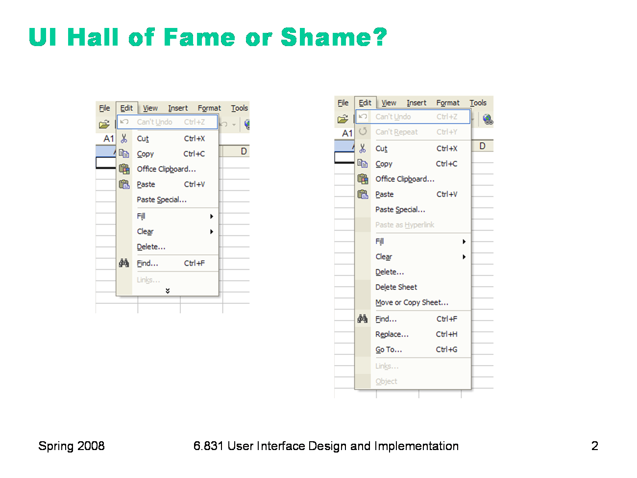
Today’s candidate for the Hall of Fame or Shame is adaptive menus, a feature of Microsoft Office 2003.  Initially, a menu shows only the most commonly used commands.  Clicking on the arrow at the bottom of the menu expands it to show all available commands. Adaptive menus track how often a user invokes each command, in order to display frequently-used commands and recently-used commands.

Let’s discuss the usability of this idea.

Here’s an alternative approach to providing easy access to high-frequency menu choices: a split menu.  You can see it in Microsoft Office’s font drop-down menu. A small number of fonts that you’ve used recently appear in the upper part of the menu, while the entire list of fonts is available in the lower part of the menu. The upper list is sorted by recency, while the lower part is sorted alphabetically.

Let’s discuss the split menu approach too.

These menu approaches are particularly relevant to today’s lecture because they’ve been compared by a controlled experiment (Sears & Shneiderman, “Split menus: effectively using selection frequency to organize menus”, ACM TOCHI, March 1994, http://doi.acm.org/10.1145/174630.174632).

Many lectures in this course have discussed various ways to test user interfaces for usability, including formative evaluation, heuristic evaluation, and predictive evaluation.  Today’s lecture covers what is sometimes called summative evaluation: establishing the usability of an interface by a rigorous controlled experiment.  This lecture covers some of the issues involved in designing such a controlled experiment. The issues are general to all scientific experiments, but we’ll look specifically at how they apply to user interface testing.  We’ll also talk a little bit about how to analyze the results of an experiment.  Doing analysis well requires statistics that is outside the scope of this course, so we’ll use some back-of-the-envelope techniques instead.

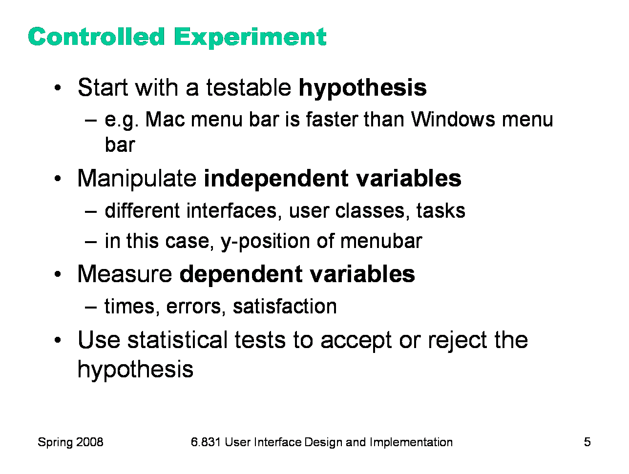
Here’s a high-level overview of a controlled experiment.  You start by stating a clear, testable hypothesis. By testable, we mean that the hypothesis must be quantifiable and measurable. Here’s an example of a hypothesis that we might want to test: that the Macintosh menu bar, which is anchored to the top of the screen, is faster to access than the Windows menu bar, which is separated from the top of the screen by a window title bar.

You then choose your independent variables — the variables you’re going to manipulate in order to test the hypothesis.  In our example, the independent variable is the kind of interface: Mac menubar or Windows menubar.  In fact, we can make it very specific: the independent variable is the y-position of the menubar (either y = 0  or y = 16, or whatever the height of the title bar is). Other independent variables may also be useful.  For example, you may want to test your hypothesis on different user classes (novices and experts, or Windows users and Mac users).  You may also want to test it on certain kinds of tasks.  For example, in one kind of task, the menus might have an alphabetized list of names; in another, they might have functionally-grouped commands.

You also have to choose the dependent variables, the variables you’ll actually measure in the experiment to test the hypothesis.  Typical dependent variables in user testing are time, error rate, event count (for events other than errors — e.g., how many times the user used a particular command), and subjective satisfaction (usually measured by numerical ratings on a questionnaire).

Finally, you use statistical techniques to analyze how your changes in the independent variables affected the dependent variables, and whether those effects are significant (indicating a genuine cause-and-effect) or not (merely the result of chance or noise). We’ll say a bit more about statistical tests later in the lecture, but note that this topic is too large for this course; you should take a statistics course to learn more.

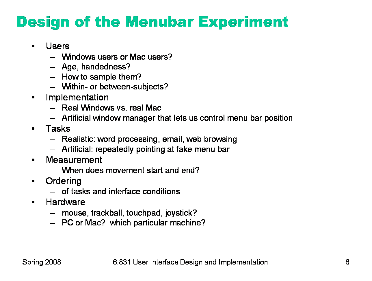
Here are some of the issues we’d have to consider in designing this study.

First, what user population do we want to sample?  Does experience matter?  Windows users will be more experienced with one kind of menu bar, and Mac users with the other.  On the other hand, the model underlying our hypothesis (Fitts’s Law) is largely independent of long-term memory or practice, so we might expect that experience doesn’t matter.  But that’s another hypothesis we should test, so maybe past experience should be an independent variable that we select when sampling.

How do we sample the user population we want?  The most common technique (in academia) is advertising around a college campus, but this biases against older users and less-educated users.  Any sampling method has biases; you have to collect demographic information, report it, and consider whether the bias influences your data.

Should this be a within-subjects or between-subjects study?  In a within-subjects study, each user will use both the Mac menu bar and the Windows menu bar; in the between-subjects study, they’ll use only one.  The biggest question here is, which is larger: individual variation between users, or learning effects between interfaces used by the same user?  A within-subjects design would probably be best here, since it has higher power, and we want to test expert usage, so learning effects should be minimized.

What implementation should we test?  One possibility is to test the menu bars in their real context: inside the Mac interface, and inside the Windows interface, using real applications and real tasks.  This is more realistic, but the problem is now the presence of confounding variables -- the size of the menu bars might be different, the reading speed of the font, the mouse acceleration parameters, etc. We need to control for as many of these variables as we can.  Another possibility is implementing our own window manager that holds these variables constant and merely changes the position of the menu bar.

What tasks should we give the user?  Again, having the user use the menu bar in the context of realistic tasks might provide more generalizable results; but it would also be noisier.  An artificial experiment that simply displays a menu bar and cues the user to hit various targets on it would provide more reliable results.  But then the user’s mouse would always be in the menu bar, which isn’t at all realistic.  We’d need to force the user to move the mouse out of the menu bar between trials, perhaps to some home location in the middle of the screen.

How do we measure the dependent variable, time? Maybe from the time the user is given the cue (“click Edit”) to the time the user successfully clicks on Edit.

What order should we present the tasks and the interface conditions? Using the same order all the time can cause both learning effects (e.g., you do better on the interface conditions because you got practice with the tasks and the study protocol during the first interface condition) and fatigue effects (where you do worse on later interface conditions because you’re getting tired).

Finally, the hardware we use for the study can introduce lots of confounding variables.  We should use the same computer for the entire experiment — across both users and interface conditions.

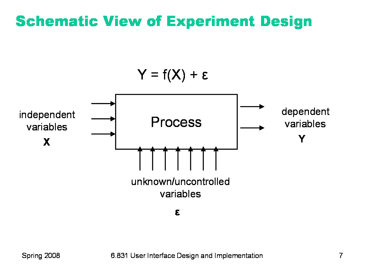
Here’s a block diagram to help you visualize what we’re trying to do with experiment design.  Think of the process you’re trying to understand (e.g., menu selection) as a black box, with lots of inputs and a few outputs.  A controlled experiment twiddles some of the input knobs on this box (the independent variables) and observes some of the outputs (the dependent variables) to see how they are affected.

The problem is that there are many other input knobs as well (unknown/uncontrolled variables), that may affect the process we’re observing in unpredictable ways.  The purpose of experiment design is to eliminate the effect of these unknown variables, or at least render harmless, so that we can draw conclusions about how the independent variables affect the dependent variables.

What are some of these unknown variables? Consider the menubar experiment.  Many factors might affect how fast the user can reach the menubar: the pointing device they’re using (mouse, trackball, isometric joystick, touchpad); where the mouse pointer started; the surface they’re moving the mouse on; the user’s level of fatigue; their past experience with one kind of menubar or the other.  All of these are unknown variables that might affect the dependent variable (speed of access).

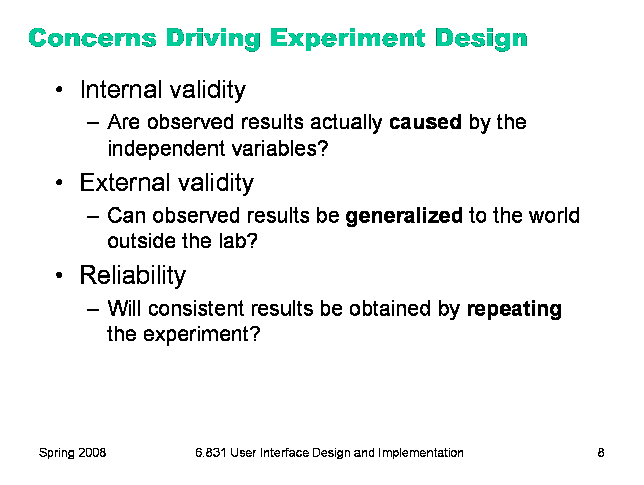
Unknown variation is the bugaboo in experiment design, and here are the three main problems it can cause.

Internal validity refers to whether the effect we see on the experiment outputs was actually caused by the changes we made to the inputs, or caused by some unknown variable that we didn’t control or measure.  For example, suppose we designed the menubar experiment so that the Mac menubar position was tested on an actual Mac, and the Windows menubar position was tested on a Windows box.  This experiment wouldn’t be internally valid, because we can’t be sure whether differences in performance were due to the difference in the position of the menubar, or to some other (unknown) difference in two machines -- like font size, mouse acceleration, mouse feel, even the system timer used to measure the performance!  Statisticians call this effect confounding; when a variable that we didn’t control has a systematic effect on the dependent variables, it’s a confounding variable.

One way to address internal validity is to hold variables constant, as much as we can: for example, conducting all user tests in the same room, with the same lighting, the same computer, the same mouse and keyboard, the same tasks, the same training. The cost of this approach is external validity, which refers to whether the effect we see can be generalized to the world outside the lab, i.e. when those variables are not controlled.  But when we try to control all the factors that might affect menu access speed — a fixed starting mouse position, a fixed menubar with fixed choices, fixed hardware, and a single user — then it would be hard to argue that our lab experiment generalizes to how menus are used in the varying conditions encountered in the real world.

Finally, reliability refers to whether the effect we see (the relationship between independent and dependent variables) is repeatable.  If we ran the experiment again, would we see the same effect?  If our experiment involved only one trial -- clicking the menubar just once — then even if we held constant every variable we could think of, unknown variations will still cause error in the experiment.  A single data sample is rarely a reliable experiment.

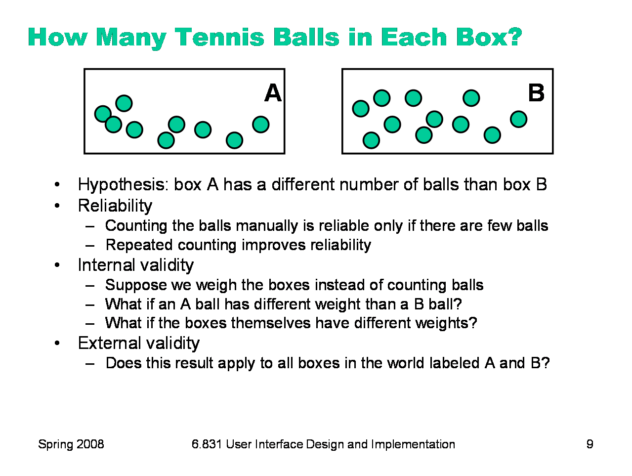
Here’s a simple example to illustrate internal validity, external validity, and reliability.

Suppose we have two boxes labeled A and B, and each box has some balls inside. We want to test the hypothesis that these two boxes have different numbers of balls.  (For example, maybe box A is a box of tennis balls from one manufacturer, and box B is a box from another manufacturer, both the same price, and we want to claim that one box is a better deal than the other.)  In this case, the independent variable is the identity of the box (the brand of the ball manufacturer), and the dependent variable we’re trying to measure is the number of balls inside the box.

This hypothesis is testable because we can do measurements on the boxes to test it.  One measurement we might do is open the boxes and count the balls inside each one.  If we counted 3 balls in one box, and 5 balls in the other box, then we’d have strong evidence that A has fewer balls than B.  But if we counted  99 balls in A and 101 balls in B, would we be just as confident?  No, because we know that our counting may have errors -- we may skip balls, or we may double-count balls.  If we counted A again, we might come up with 102 balls.  The reliability of a single measurement isn’t good enough. We can fix this reliability problem by better experiment design: counting each box several times, and computing a statistic (a summary of the measurements) instead of using a single measurement.  The statistic is often the mean of the measurements, but others are possible.

Counting is pretty slow, though, so to make our experiment cheaper to run, suppose we weigh the boxes instead.  If box A is lighter than box B, then we’ll say that it has fewer balls in it.  It’s easy to see the possible flaws in this experiment design: what if each ball in box A is lighter than each ball in box B?  Then the whole box A might be lighter than B even if it has more balls.  If this is true, then it threatens the experiment’s internal validity: the dependent variable we’ve chosen to measure (total weight) is a function not only of the number of balls in the box, but also of the weight of each ball, and the weight of the ball also varies by the independent variable (the identity of the box).

Suppose the weight of tennis balls is regulated by an international standard, so we can argue that A balls should weigh the same as B balls.  But what if box A is made out of metal, and box B is made out of cardboard?  This would also threaten internal validity — the weight of the box itself is a confounding variable.  But now we can imagine a way to control for this variable, by pouring the balls out of their original boxes into box C, a box that we’ve chosen, and weighing both sets of balls separately in box C.  We’ve changed our experiment design so that the weight of the box itself is held constant, so that it won’t contribute to the measured difference between box A and box B.

But we’ve only done this experiment with the box A and box B we have in front of us.  What confidence do we have in concluding that all boxes from manufacturer A have a different number of balls than those from manufacturer B — that if we went to the store and picked up new boxes of balls, we’d see the same difference?  That’s the question of external validity.

Let’s look closer at typical dangers to internal validity in user interface experiments, and some solutions to them.  You’ll notice that the solutions come in two flavors: randomization (which prevents unknown variables from having systematic effects on the dependent variables) and control (which tries to hold unknown variables constant).

Ordering effects refer to the order in which different levels of the independent variables are applied.  For example, does the user work with interface X first, and then interface Y, or vice versa?  There are two effects from ordering: first, people learn.  They may learn something from using interface X that helps them do better (or worse) with interface Y.  Second, people get tired or bored.  After doing many tasks with interface X, they may not perform as well on interface Y. Clearly, holding the order constant threatens internal validity, because the ordering may be responsible for the differences in performance, rather than inherent qualities of the interfaces.  The solution to this threat is randomization: present the interfaces, or tasks, or other independent variables in a random order to each user.

Selection effects arise when you use pre-existing groups as a basis for assigning different levels of an independent variable.  Giving the Mac menubar to artists and the Windows menubar to engineers would be an obvious selection effect.  More subtle selection effects can arise, however.  Suppose you let the users line up, and then assigned the Mac menubar to the first half of the line, and Windows menubar to the second half.  This procedure seems “random”, but it isn’t — the users may line up with their friends, and groups of friends tend to have similar activities and interests.  The same thing can happens even if people are responding “randomly” to your study advertisement — you don’t know how “random” that really is!  The only safe way to eliminate selection effects is honest randomization.

A third important threat to internal validity is experimenter bias.  After all, you have a hypothesis, and you’re hoping it works out — you’re rooting for interface X.  This bias is an unknown variable that may affect the outcome, since you’re personally interacting with the user whose performance you’re measuring.  One way to address experimenter bias is controlling the protocol of the experiment, so that it doesn’t vary between the interface conditions. Provide equivalent training for both interfaces, and give it on paper, not live.

An even better technique for eliminating experimenter bias is the double-blind experiment, in which neither the subject nor the experimenter knows which condition is currently being tested.  Double-blind experiments are the standard for clinical drug trials, for example; neither the patient nor the doctor knows whether the pill contains the actual experimental drug, or just a placebo. With user interfaces, double-blind tests may be impossible, since the interface condition is often obvious on its face.  (Not always, though!  The behavior of cascading submenus isn’t obviously visible.)

Experimenter-blind tests are essential if measurement of the dependent variables requires some subjective judgement. Suppose you’re  developing an interface that’s supposed to help people compose good memos. To measure the quality of the resulting memos, you might ask some people to evaluate the memos created with the interface, along with memos created with a regular word processor.  But the memos should be presented in random order, and you should hide the interface that created each memo from the judge, to avoid bias.

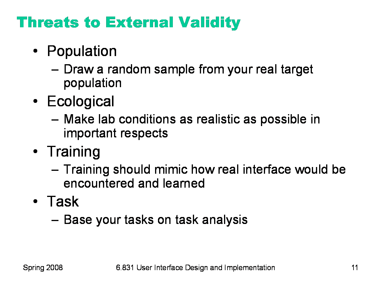
Here are some threats to external validity that often come up in user studies.  If you’ve done a thorough user analysis and task analysis, in which you actually went out and observed the real world, then it’s easier to judge whether your experiment is externally valid.

Population asks whether the users you sampled are representative of the target user population.  Do your results apply to the entire user population, or only to the subgroup you sampled?  The best way to ensure population validity is to draw a random sample from your real target user population.  But you can’t really, because users must choose, of their own free will, whether or not to participate in a study.  So there’s a self-selection effect already in action.  The kinds of people who participate in user studies may have special properties (extroversion? curiosity? sense of adventure? poverty?) that threaten external validity.  But that’s an inevitable effect of the ethics of user testing.  The best you can do is argue that on important, measurable variables — demographics, skill level, experience — your sample resembles the overall target user population.

Ecological validity asks whether conditions in the lab are like the real world.  An office environment would not be an ecologically valid environment for studying an interface designed for the dashboard of a car, for example.

Training validity asks whether the interfaces tested are presented to users in a way that’s realistic to how they would encounter them in the real world. A test of an ATM machine that briefed each user with a 5-minute tutorial video wouldn’t be externally valid, because no ATM user in the real world would watch such a video.  For a test of an avionics system in an airplane cockpit, on the other hand, even hours of tutorial may be externally valid, since pilots are highly trained.

Similarly, task validity refers to whether the tasks you chose are realistic and representative of the tasks that users actually face in the real world.  If you did a good task analysis, it’s not hard to argue for task validity.

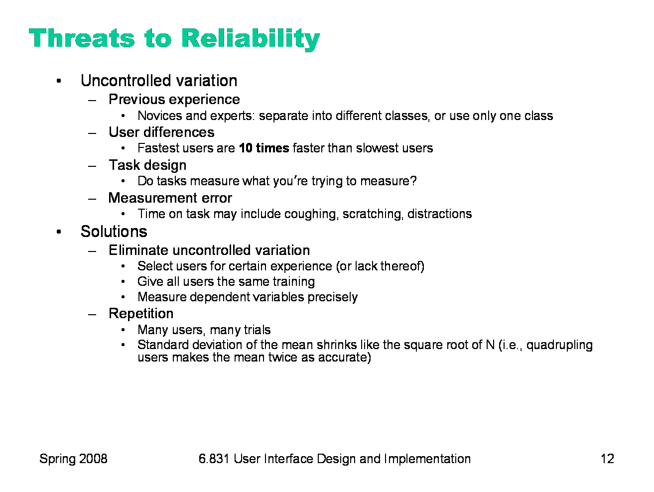
Once we’ve addressed internal validity problems by either controlling or randomizing the unknowns, and external validity by sampling and experiment protocol design, reliability is what’s left.

Here’s a good way to visualize reliability: imagine a bullseye target.  The center of the bullseye is the true effect that the independent variables have on the dependent variables.  Using the independent variables, you try to aim at the center of the target, but the uncontrolled variables are spoiling your aim, creating a spread pattern. If you can reduce the amount of uncontrolled variation, you’ll get a tighter shot group, and more reliable results.

One kind of uncontrolled variation is a user’s previous experience.  Users enter your lab with a whole lifetime of history behind them, not just interacting with computers but interacting with the real world.  You can limit this variation somewhat by screening users for certain kinds of experience, but take care not to threaten external validity when you artificially restrict your user sample.

Even more variation comes from differences in ability — intelligence, visual acuity, memory, motor skills.  The best users may be 10 times better than the worst, an enormous variation that may swamp a tiny effect you’re trying to detect.

Other kinds of uncontrolled variation arise when you can’t directly measure the dependent variables.  For example, the tasks you chose to measure may have their own variation, such as the time to understand the task itself, and errors due to misunderstanding the task, which aren’t related to the difficulty of the interface and act only to reduce the reliability of the test. Time is itself a gross measurement which may include lots of activities unrelated to the user interface: coughing, sneezing, asking questions, responding to distractions.

One way to improve reliability eliminates uncontrolled variation by holding variables constant: e.g., selecting users for certain experience, giving them all identical training, and carefully controlling how they interact with the interface so that you can measure the dependent variables precisely.  If you control too many unknowns, however, you have to think about whether you’ve made your experiment externally invalid, creating an artificial situation that no longer reflects the real world.

The main way to make an experiment reliable is repetition.  We run many users, and have each user do many trials, so that the mean of the samples will approach the bullseye we want to hit.  As you may know from statistics, the more trials you do, the closer the sample mean is likely to be to the true value. (Assuming the experiment is internally valid of course!  Otherwise, the mean will just get closer and closer to the wrong value.)  Unfortunately, the standard deviation of the sample mean goes down slowly, proportionally to the square root of the number of samples N.  So you have to quadruple the number of users, or trials, in order to double reliability.

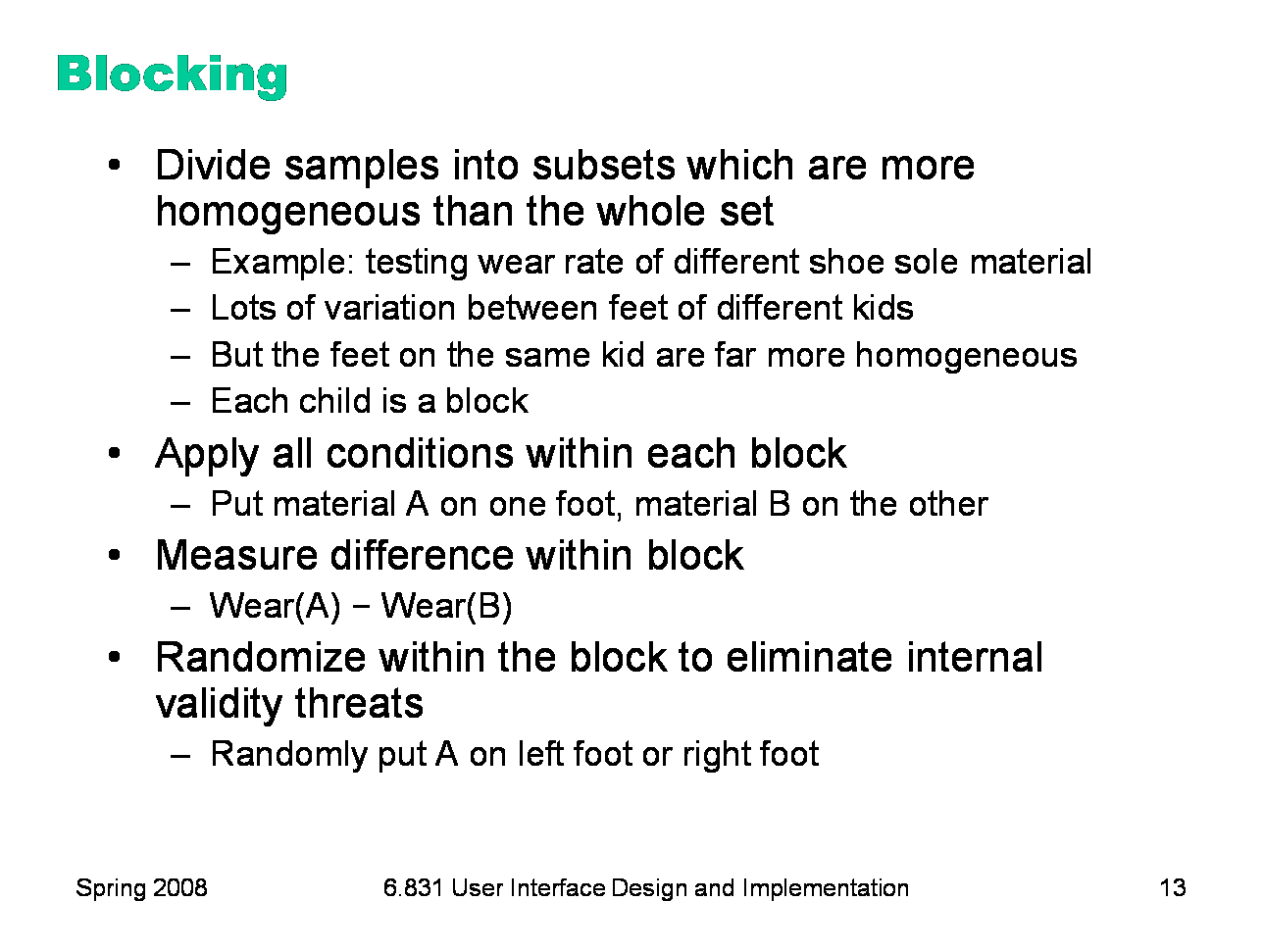
Blocking is another good way to eliminate uncontrolled variation, and therefore increase reliability.  The basic idea is to divide up your samples up into blocks that are more homogeneous than the whole set.  In other words, even if there is lots of uncontrolled variation between blocks, the blocks should be chosen so that there is little variation within a block.  Once you’ve blocked your data, you apply all the independent variable conditions within each block, and compare the dependent variables only within the block.

Here’s a simple example of blocking.  Suppose you’re studying materials for the soles of childrens’ shoes, and you want to see if material A wears faster or slower than material B. There’s much uncontrolled variation between feet of different children — how they behave, where they live and walk and play — but the two feet of the same child both see very similar conditions by comparison. So we treat each child as a block, and apply one sole material to one foot, and the other sole material to the other foot.  Then we measure the difference between the sole wear as our dependent variable.  This technique prevents inter-child variation from swamping the effect we’re trying to see.

In agriculture, blocking is done in space.  A field is divided up into small plots, and all the treatments (pesticides, for example) are applied to plants in each plot.  Even though different parts of the field may differ widely in soil quality, light, water, or air quality, plants in the same plot are likely to be living in very similar conditions.

Blocking helps solve reliability problems, but it doesn’t address internal validity.  What if we always assigned material A to the left foot, and material B to the right foot?  Since most people are right-handed and left-footed, some of the difference in sole wear may be caused by footedness, and not by the sole material.  So you should still randomize assignments within the block.

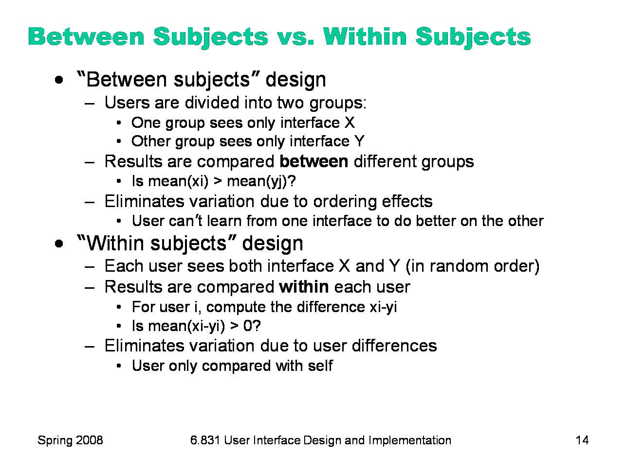
The idea of blocking is what separates two commonly-used designs in user studies that compare two interfaces.  Looking at these designs also gives us an opportunity to review some of the concepts we’ve discussed in this lecture.

A between-subjects design is unblocked.  Users are randomly divided into two groups.  These groups aren’t blocks!  Why? First, because they aren’t more homogeneous than the whole set — they were chosen randomly, after all.  And second, because we’re going to apply only one independent variable condition within each group. One group uses only interface X, and the other group uses only interface Y.  The mean performance of the X group is then compared with the mean performance of the Y group.  This design eliminates variation due to interface ordering effects.  Since users only see one interface, they can’t transfer what they learned from one interface to the other, and they won’t be more tired on one interface than the other.  But it suffers from reliability problems, because the differences between the interfaces may be swamped by the innate differences between users.  As a result, you need more repetition — more users — to get reliable and significant results from a between subjects design.

A within-subjects design is blocked by user.  Each user sees both interfaces, and the differential performance (performance on X — performance on Y) of all users is averaged and compared with 0.  This design eliminates variation due to user differences, but may have reliability problems due to ordering effects.

Which design is better? User differences cause much more variation than ordering effects, so the between-subjects design needs more users than the within-subjects design.  But the between-subjects design may be more externally valid.

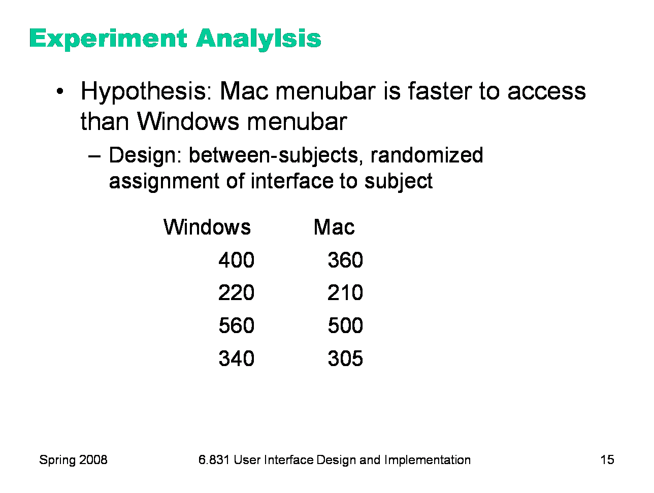
Suppose we’ve conducted an experiment to compare the position of the Mac menubar (flush against the top of the screen) with the Windows menubar (separated from the top by a window title bar).

For the moment, let’s suppose we used a between-subjects design.  We recruited users, and each user used only one version of the menu bar, and we’ll be comparing different users’ times. For simplicity, each user did only one trial, clicking on the menu bar just once while we timed their speed of access.  The results of the experiment are shown above (times in milliseconds).  Mac seems to be faster (343.75 ms on average) than Windows (380 ms).  But given the noise in the measurements — some of the Mac trials are actually much slower than some of the Windows trials -- how do we know whether the Mac menubar is really faster?

This is the fundamental question underlying statistical analysis: estimating the amount of evidence in support of our hypothesis, even in the presence of noise.

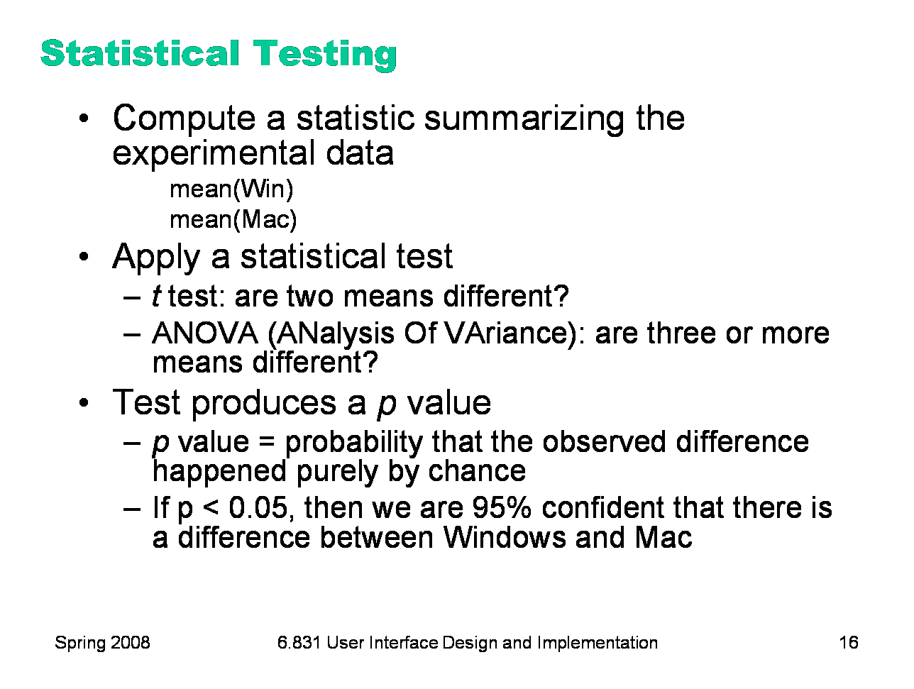
Here’s the basic process we follow to determine whether the measurements we made support the hypothesis or not.

We summarize the data with a statistic (which, by definition, is just that: a function computed from a set of data samples).  A common statistic is the mean of the data, but it’s not necessarily the only useful one.  Depending on what property of the process we’re interesting in measuring, we may also compute the variance (or standard deviation), or median, or mode (the most frequent value).  Some researchers argue that for human behavior, the median is a better statistic than the mean, because the mean is far more distorted by outliers (people who are very slow or very fast, for example) than the median.

Then we apply a statistical test that tells us whether the statistics support our hypothesis.  Two common tests for means are the t test (which asks whether the mean of one condition is different from the mean of another condition) and ANOVA (which asks the same question when we have the means of three or more conditions).

The statistical test produces a p value, which is the probability that the difference in statisics that we observed happened purely by chance.  Every run of an experiment has random noise; the p value is basically the probability that the means were different only because of these random factors.  Thus, if the p value is less than 0.05, then we have a 95% confidence that there really is a difference.

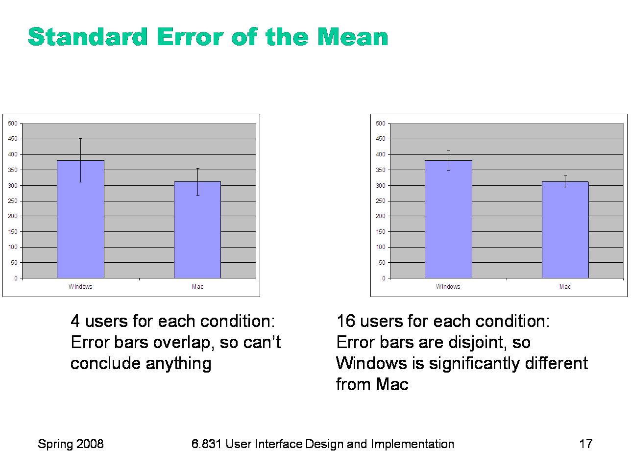
The details of how the t test and ANOVA tests work are outside the scope of this course.  (A good course for this is 9.07, Statistical Methods in Brain & Cognitive Sciences.)  But we can talk about a simpler method for judging whether an experiment supports its hypothesis or not, if the statistics you’re using are means.

The standard error of the mean is a statistic that measures how close the mean statistic you computed is likely to be to the true mean.  The standard error is computed by taking the standard deviation of the measurements and dividing by the square root of n, the number of measurements.    (This is derived from the Central Limit Theorem of probability theory: that the sum of N samples from a distribution with mean u and variance V has a probability distribution that approaches a normal distribution, i.e. a bell curve, whose mean is Nu and whose variance is V.  Thus, the average of the N samples would have a normal distribution with mean u and variance V/n.  Its standard deviation would be sqrt(V/N), or equivalently, the standard deviation of the underlying distribution divided by sqrt(n).)

The standard error is a confidence interval for your computed mean. Think of your computed mean as a random selection from a normal distribution (bell curve) around the true mean; it’s random because of all the uncontrolled variables and intentional randomization that you did in your experiment. With a normal distribution, 68% of the time your random sample will be within +/-1 standard deviation of the mean; 95% of the time it will be within +/- 2 standard deviations of the mean.  The standard error is the standard deviation of the mean’s normal distribution, so what this means is that if we draw an error bar one standard error above our computed mean, and one standard error below our computed mean, then that interval will have the true mean in it 68% of the time.  It is therefore a 68% confidence interval for the mean.

If we draw the error bar for both computed means — Windows and Mac — and look at whether those error bars overlap or are substantially different, then we can make a quick judgement about whether the true means are likely to be different.  Suppose the error bars overlap — then it’s possible that the true means  for both conditions are actually the same — in other words, that whether you use the Windows or Mac menubar design makes no difference to the speed of access.  But if the error bars do not overlap, then it’s very likely that the true means are different.  (How likely?  Suppose the true mean lies somewhere between the two error bars, but outside both of them.  Then the probability of seeing the results you did — your computed means so far away from the true mean — is 1-(1-0.68)*(1-0.68), which is about 10%.)

The error bars can also give you a sense about the reliability of your experiment, also called the statistical power.  If you didn’t take enough samples, your error bars will be large relative to the size of the data.  So the error bars may overlap even though there really is a difference between the conditions.  The solution is more repetition — more trials and/or more users — in order to increase the reliability of the experiment.

Plotting your data with error bars is the first step you should do after every experiment, to eyeball your results and judge whether statistical testing is worthwhile, or whether you need more data.  If you want to publish the results of your experiment, you’ll probably need to do some statistical tests as well, like t tests or ANOVAs.  But your paper should still have plots with error bars in it.  Some researchers even argue that the error-bar plots are more valuable and persuasive than the statistical tests (G.R. Loftus, “A picture is worth a thousand p values: On the irrelevance of hypothesis testing in the microcomputer age,” Behavior Research Methods, Instruments & Computers, 1993, 25(2), 250—256).