To print these notes, use the PDF version.

From Daniel Gutierrez:

“The speed dial implemented into the Opera web browser (screen shot attached) is designed to provide a type of visual bookmark for quick access to web pages.  It appears in a newly created tab and begins to load each of the websites to create a preview thumbnail for each one.  When you click on any of these, it navigates the browser to the web page.  One cool thing about this is that it actually starts to cache images and similar content from the websites it’s loading while the browser is idling on this screen.”

Let’s talk about this interface in terms of:

- visibility

- efficiency

- graphic design

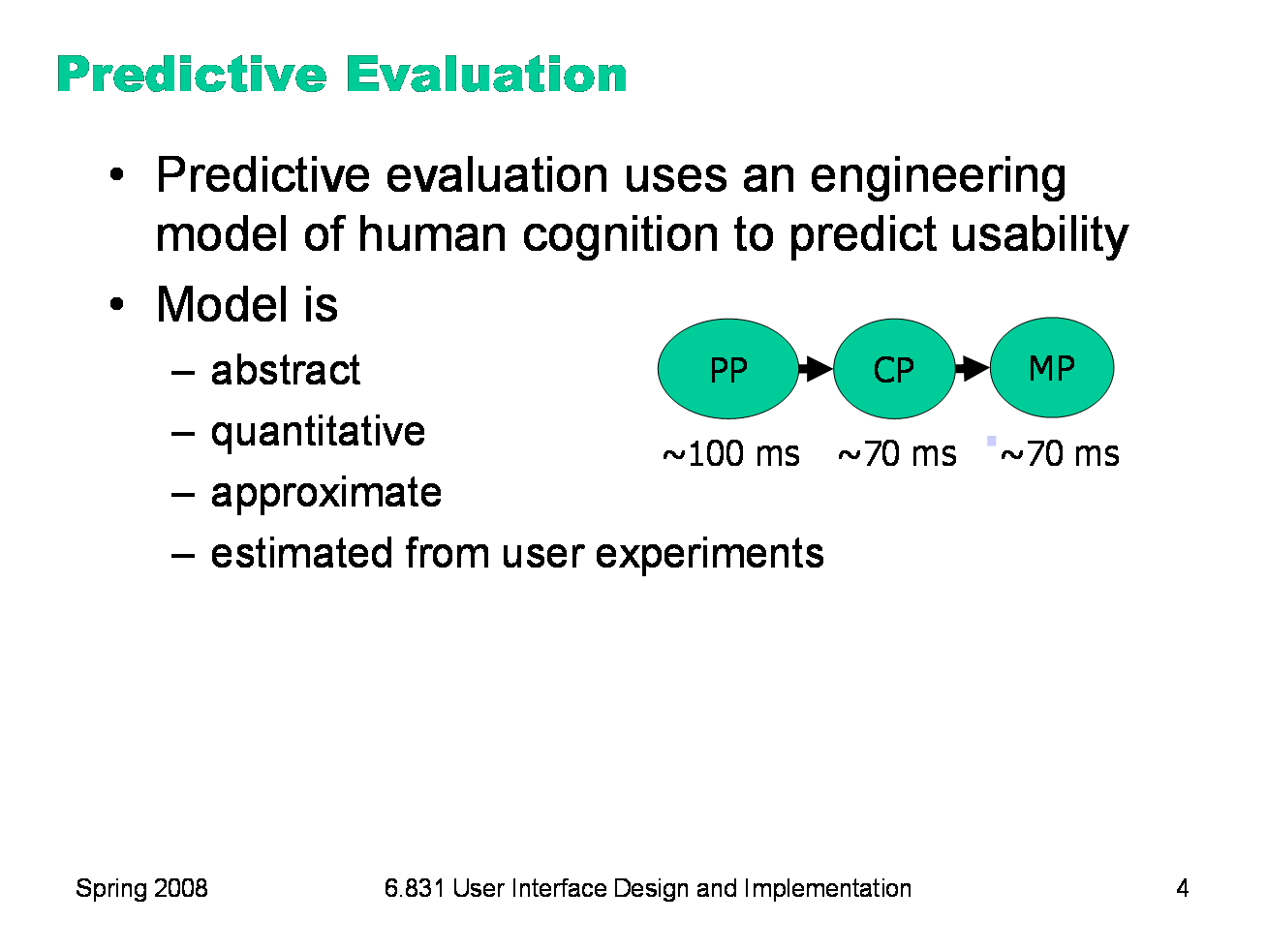
Today’s lecture is about predictive evaluation — the holy grail of usability engineering.  If we had an accurate model for the way a human used a computer interface, we would be able to predict the usability of a design, without having to actually build it, test it against real people, and measure their behavior.  User interface design would then become more like other fields of engineering.  Civil engineers can use models (of material stress and strain) to predict the load that can be carried by a bridge; they don’t have to build it and test it to destruction first.  As user interface designers, we’d like to do the same thing.

At its heart, any predictive evaluation technique requires a model for how a user interacts with an interface.  We’ve already seen one such model, the Newell/Card/Moran human information processing model. 

This model needs to be abstract — it can’t be as detailed as an actual human being (with billions of neurons, muscles, and sensory cells), because it wouldn’t be practical to use for prediction. The model we looked at boiled down the rich aspects of information processing into just three processors and two memories.

It also has to be quantitative, i.e., assigning numerical parameters to each component.  Without parameters, we won’t be able to compute a prediction. We might still be able to do qualitative comparisons, such as we’ve already done to compare, say, Mac menu bars with Windows menu bars, or cascading submenus.  But our goals for predictive evaluation are more ambitious.

These numerical parameters are necessarily approximate; first because the abstraction in the model aggregates over a rich variety of different conditions and tasks; and second because human beings exhibit large individual differences, sometimes up to a factor of 10 between the worst and the best.  So the parameters we use will be averages, and we may want to take the variance of the parameters into account when we do calculations with the model.

Where do the parameters come from?  They’re estimated from experiments with real users.  The numbers seen here for the general model of human information processing (e.g., cycle times of processors and capacities of memories) were inferred from a long literature of cognitive psychology experiments.  But for more specific models, parameters may actually be estimated by setting up new experiments designed to measure just that parameter of the model.

Predictive evaluation doesn’t need real users (once the parameters of the model have been estimated, that is).  Not only that, but predictive evaluation doesn’t even need a prototype. Designs can be compared and evaluated without even producing design sketches or paper prototypes, let alone code.

Another key advantage is that the predictive evaluation not only identifies usability problems, but actually provides an explanation of them based on the theoretical model underlying the evaluation.  So it’s much better at pointing to solutions to the problems than either inspection techniques or user testing.  User testing might show that design A is 25% slower than design B at a doing a particular task, but it won’t explain why.  Predictive evaluation breaks down the user’s behavior into little pieces, so that you can actually point at the part of the task that was slower, and see why it was slower.

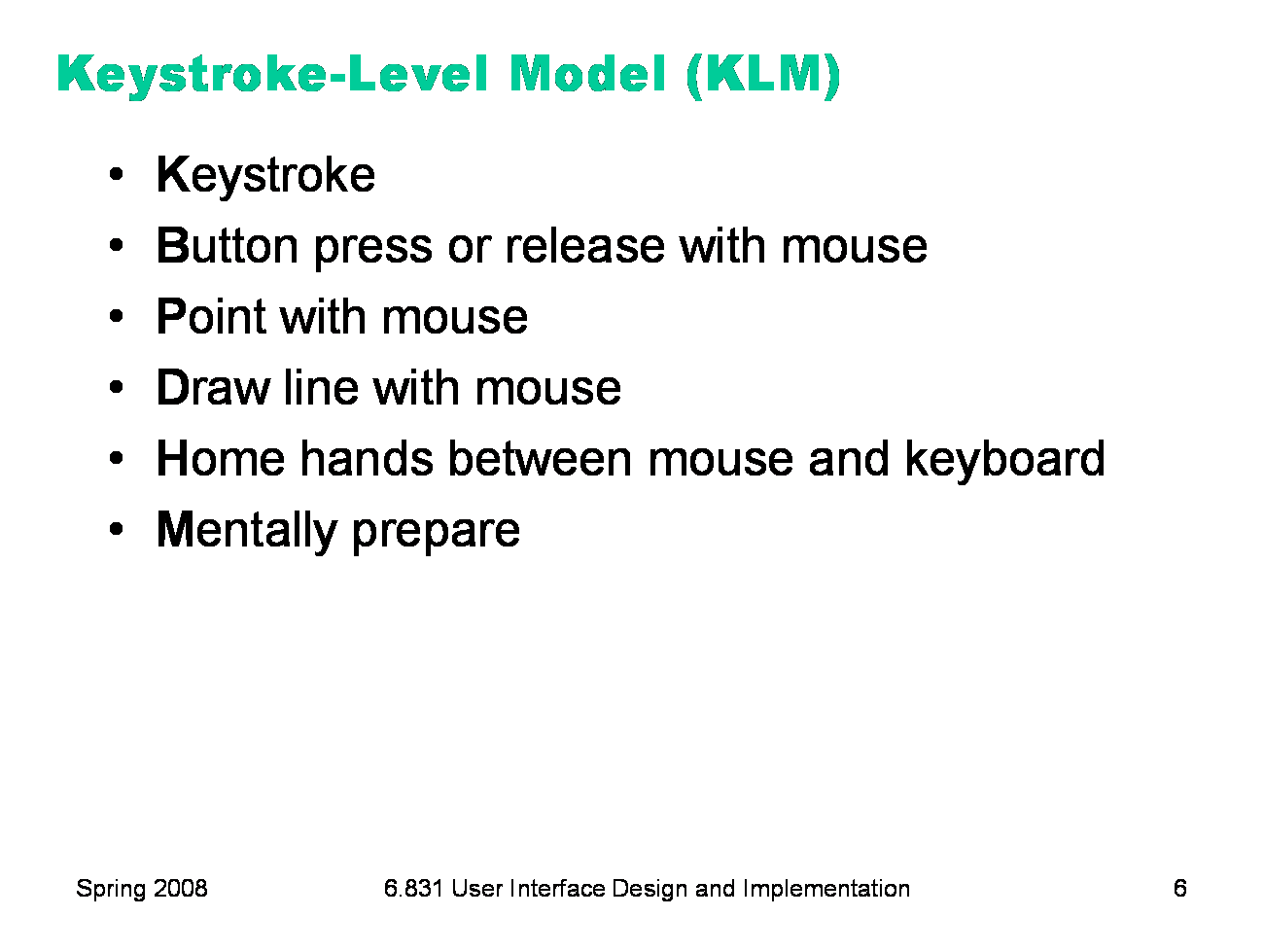
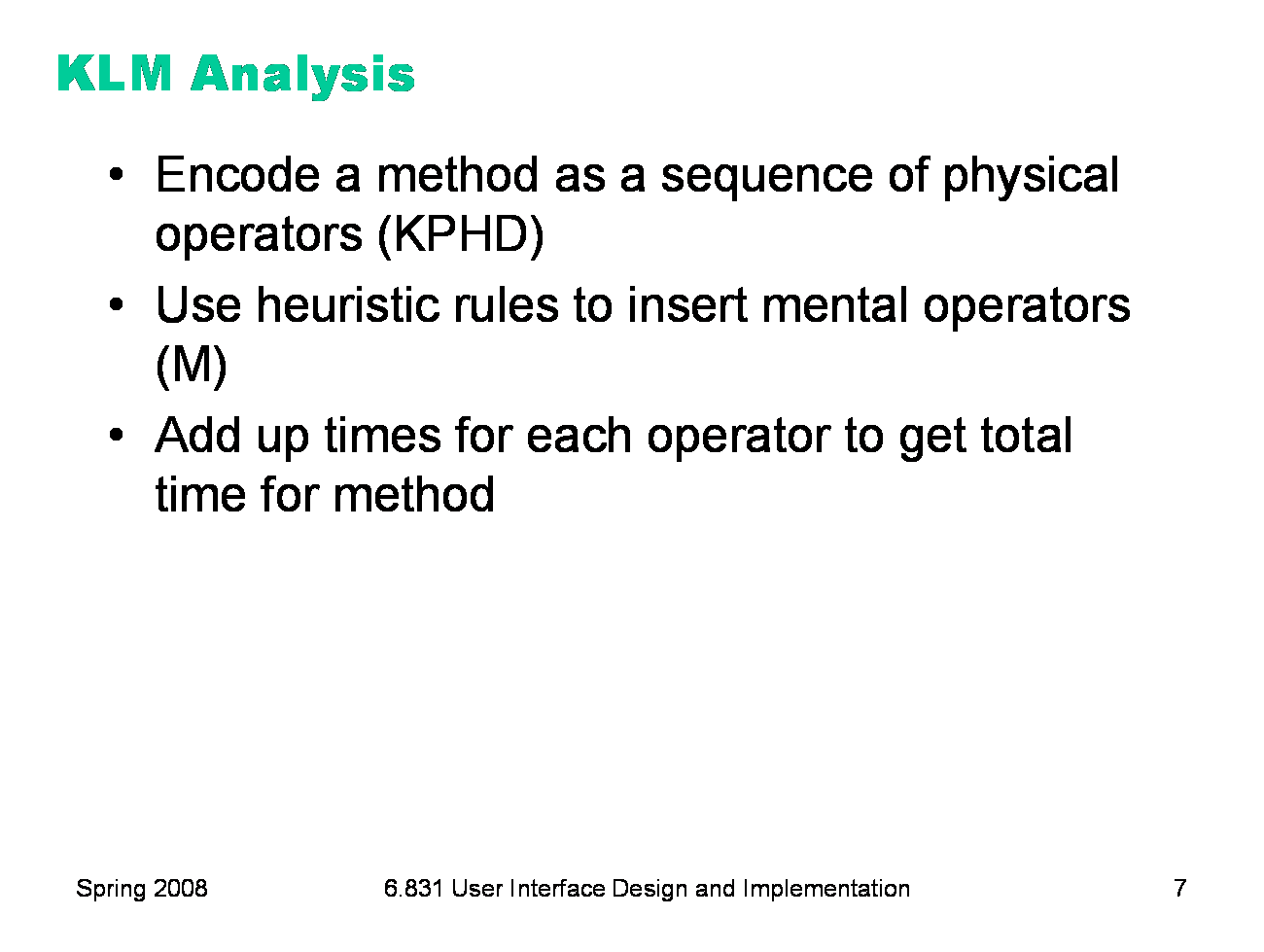
The first predictive model was the keystroke level model (proposed by Card, Moran & Newell, “The Keystroke Level Model for User Performance Time with Interactive Systems”, CACM, v23 n7, July 1978).

This model seeks to predict efficiency (time taken by expert users doing routine tasks) by breaking down the user’s behavior into a sequence of the five primitive operators shown here.

Most of the operators are physical — the user is actually moving their muscles to perform them.  The M operator is different — it’s purely mental (which is somewhat problematic, because it’s hard to observe and estimate).  The M operator stands in for any mental operations that the user does.  M operators separate the task into chunks, or steps, and represent the time needed for the user to recall the next step from long-term memory.

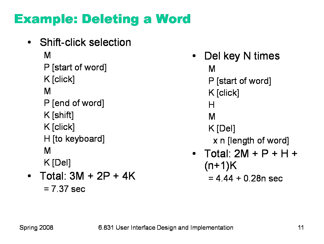
Here’s how to create a keystroke level model for a task.

First, you have to focus on a particular method for doing the task.  Suppose the task is deleting a word in a text editor.  Most text editors offer a variety of methods for doing this, e.g.: (1) click and drag to select the word, then press the Del key; (2) click at the start and shift-click at the end to select the word, then press the Del key; (3) click at the start, then press the Del key N times; (4) double-click the word, then select the Edit/Delete menu command; etc. 

Next, encode the method as a sequence of the physical operators: K for keystrokes, B for mouse button presses or releases, P for pointing tasks, H for moving the hand between mouse and keyboard, and D for drawing tasks.

Next, insert the mental preparation operators at the appropriate places, before each chunk in the task.  Some heuristic rules have been proposed for finding these chunk boundaries.

Finally, using estimated times for each operator, add up all the times to get the total time to run the whole method.

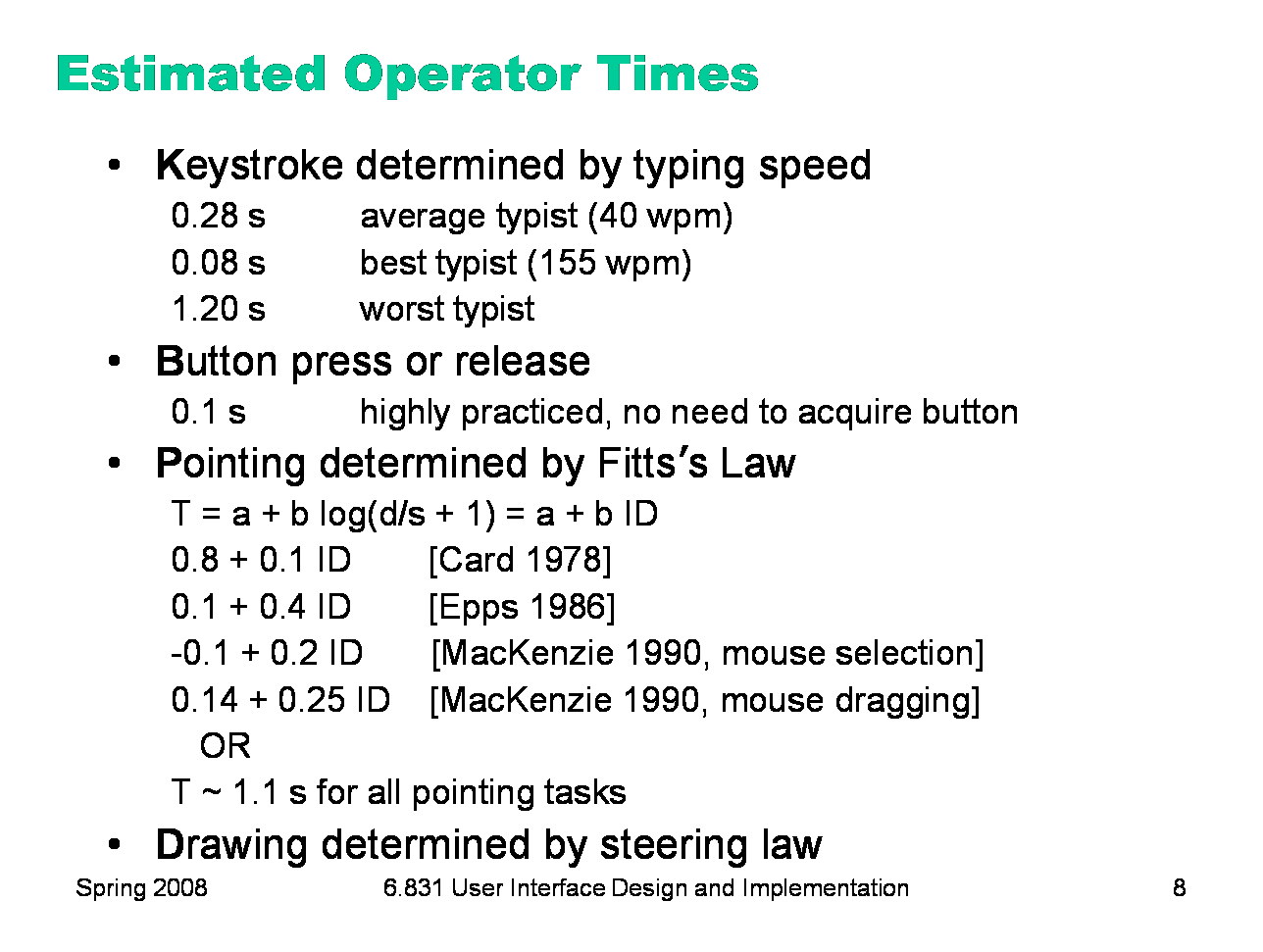
The operator times can be estimated in various ways.

Keystroke time can be approximated by typing speed. Second, if we use only an average estimate for K, we’re ignoring the 10x individual differences in typing speed.

Button press time is approximately 100 milliseconds. Mouse buttons are faster than keystrokes because there are far fewer mouse buttons to choose from (reducing the user’s reaction time) and they’re right under the user’s fingers (eliminating lateral movement time), so mouse buttons should be faster to press. Note that a mouse click is a press and a release, so it costs 0.2 seconds in this model.

Pointing time can be modelled by Fitts’s Law, but now we’ll actually need numerical parameters for it.  Empirically, you get a better fit to measurements if the index of difficulty is log(D/S+1); but even then, differences in pointing devices and methods of measurement have produced wide variations in the parameters (some of them seen here).  There’s even a measurable difference between a relaxed hand (no mouse buttons pressed) and a tense hand (dragging).  Also, using Fitts’s Law depends on keeping detailed track of the location of the mouse pointer in the model, and the positions of targets on the screen.  An abstract model like the keystroke level model dispenses with these details and just assumes that Tp ~ 1.1s for all pointing tasks.  If your design alternatives require more detailed modeling, however, you would want to use Fitts’s Law more carefully.

Drawing time, likewise, can be modeled by the steering law: T = a + b (D/S).

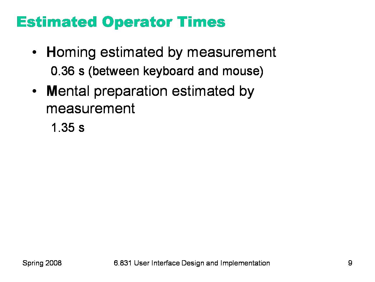
Homing time is estimated by a simple experiment in which the user moves their hand back and forth from the keyboard to the mouse.

Finally we have the Mental operator.  The M operator does not represent planning, problem solving, or deep thinking.  None of that is modeled by the keystroke level model.  M merely represents the time to prepare mentally for the next step in the method — primarily to retrieve that step (the thing you’ll have to do) from long-term memory.  A step is a chunk of the method, so the M operators divide the method into chunks. 

The time for each M operator was estimated by modeling a variety of methods, measuring actual user time on those methods, and subtracting the time used for the physical operators — the result was the total mental time.  This mental time was then divided by the number of chunks in the method.  The resulting estimate (from the 1978 Card & Moran paper) was 1.35 sec — unfortunately large, larger than any single physical operator, so the number of M operators inserted in the model may have a significant effect on its overall time.  (The standard deviation of M among individuals is estimated at 1.1 sec, so individual differences are sizeable too.)

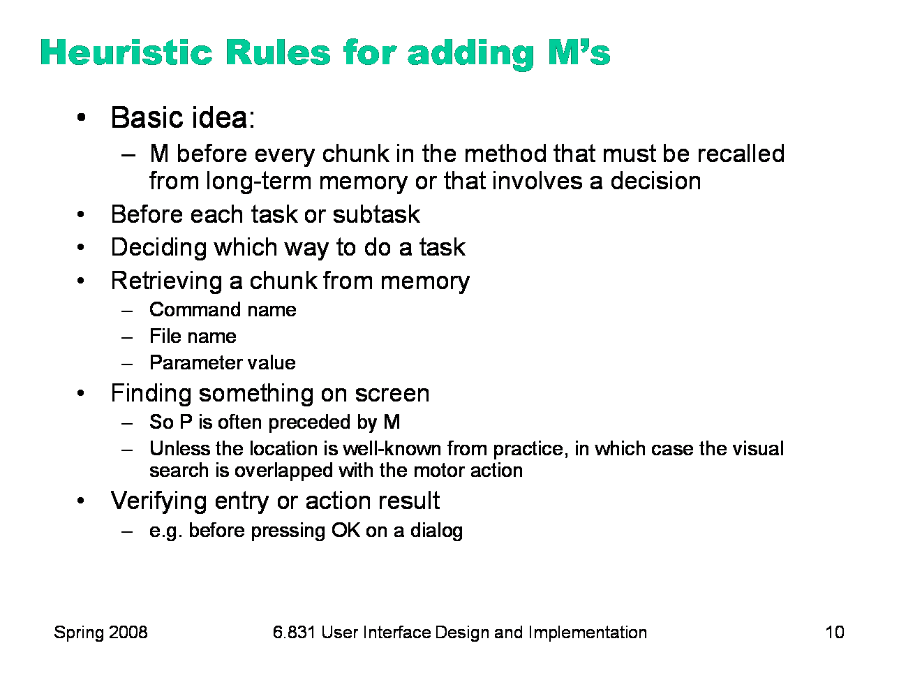
One of the trickiest parts of keystroke-level modeling is figuring out where to insert the M’s, because it’s not always clear where the chunk boundaries are in the method.  Here are some heuristic rules, suggested by Kieras (“Using the Keystroke-Level Model to Estimate Execution Times”, 2001).

Here are keystroke-level models for two methods that delete a word.

The first method clicks at the start of the word, shift-clicks at the end of the word to highlight it, and then presses the Del key on the keyboard.  Notice the H operator for moving the hand from the mouse to the keyboard.  That operator may not be necessary if the user uses the hand already on the keyboard (which pressed Shift) to reach over and press Del.

The second method clicks at the start of the word, then presses Del enough times to delete all the characters in the word.

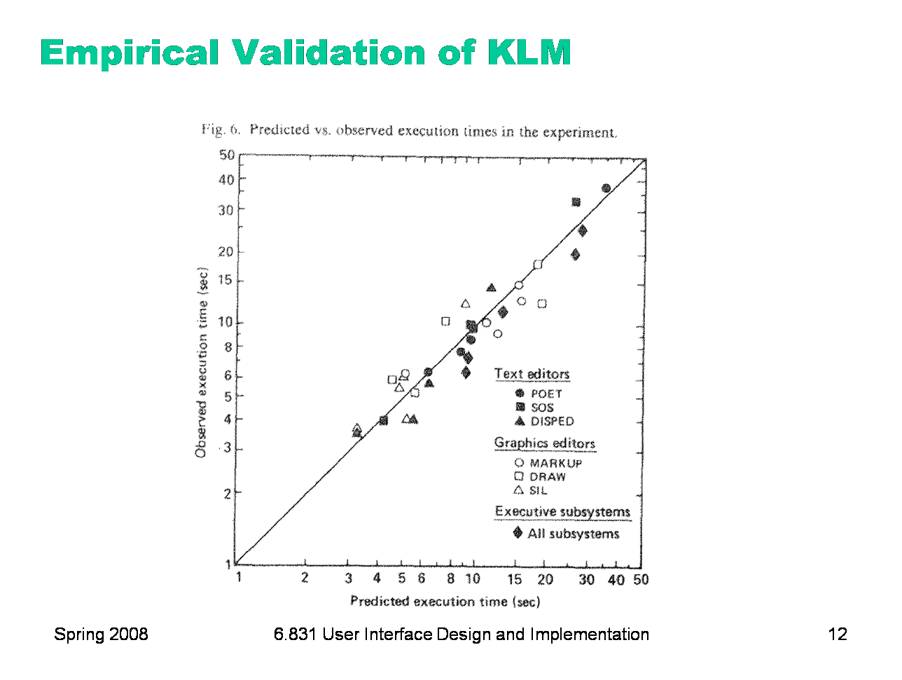
The developers of the KLM model tested it by comparing its predications against the actual performance of users on 11 different interfaces (3 text editors, 3 graphical editors, and 5 command-line interfaces like FTP and chat). 

28 expert users were used in the test (most of whom used only one interface, the one they were expert in).

The tasks were diverse but simple: e.g. substituting one word with another; moving a sentence to the end of a paragraph; adding a rectangle to a diagram; sending a file to another computer.  Users were told the precise method to use for each task, and given a chance to practice the method before doing the timed tasks.

Each task was done 10 times, and the observed times are means of those tasks over all users.

The results are pretty close — the predicted time for most tasks is within 20% of the actual time.  (To give you some perspective, civil engineers usually expect that their analytical models will be within 20% error in at least 95% of cases, so KLM is getting close to that.)

One flaw in this study is the way they estimated the time for mental operators — it was estimated from the study data itself, rather than from separate, prior observations.

For more details, see the paper from which this figure was taken: Card, Moran & Newell, “The Keystroke Level Model for User Performance Time with Interactive Systems”, CACM, v23 n7, July 1978.

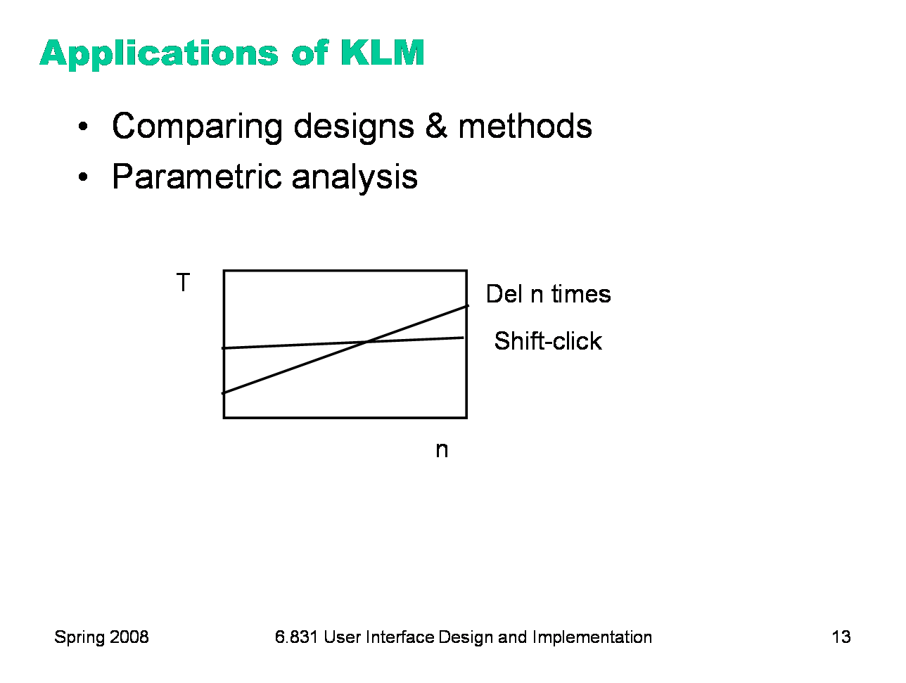
Keystroke level models can be useful for comparing efficiency of different user interface designs, or of different methods using the same design.

One kind of comparison enabled by the model is parametric analysis — e.g., as we vary the parameter n (the length of the word to be deleted), how do the times for each method vary?

Using the approximations in our keystroke level model, the shift-click method is roughly constant, while the Del-n-times method is linear in n.  So there will be some point n below which the Del key is the faster method, and above which Shift-click is the faster method.  Predictive evaluation not only tells us that this point exists, but also gives us an estimate for n.

But here the limitations of our approximate models become evident.  The shift-click method isn’t really constant with n — as the word grows, the distance you have to move the mouse to click at the end of the word grows likewise. Our keystroke-level approximation hasn’t accounted for that, since it assumes that all P operators take constant time.  On the other hand, Fitts’s Law says that the pointing time would grow at most logarithmically with n, while pressing Del n times clearly grows linearly.  So the approximation may be fine in this case.

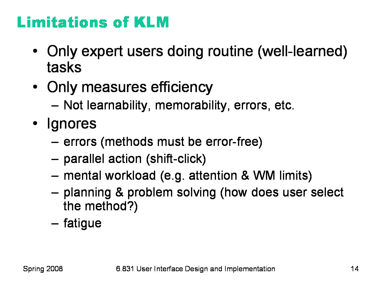
Keystroke level models have some limitations -- we’ve already discussed the focus on expert users and efficiency.  But KLM also assumes no errors made in the execution of the method, which isn’t true even for experts.  Methods may differ not just in time to execute but also in propensity of errors, and KLM doesn’t account for that.

KLM also assumes that all actions are serialized, even actions that involve different hands (like moving the mouse and pressing down the Shift key).  Real experts don’t behave that way; they overlap operations.

KLM also doesn’t have a fine-grained model of mental operations.  Planning, problem solving, different levels of working memory load can all affect time and error rate; KLM lumps them into the M operator.

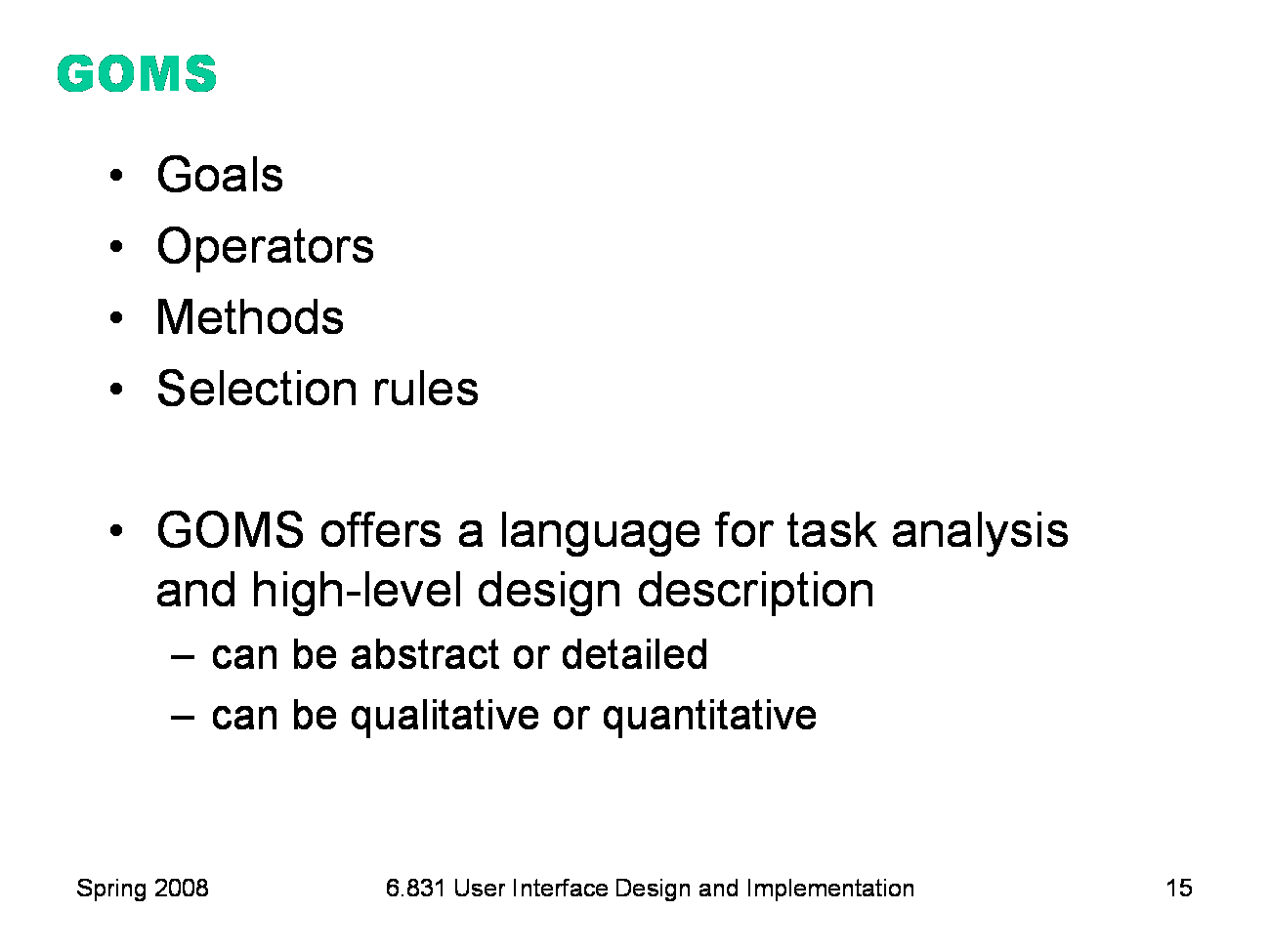
GOMS is a richer model that considers the planning and problem solving steps.  Starting with the low-level Operators and Methods provided by KLM, GOMS adds on a hierarchy of high-level Goals and subgoals (like we looked at for task analysis) and Selection rules that determine how the user decides which method will be used to satisfy a goal.

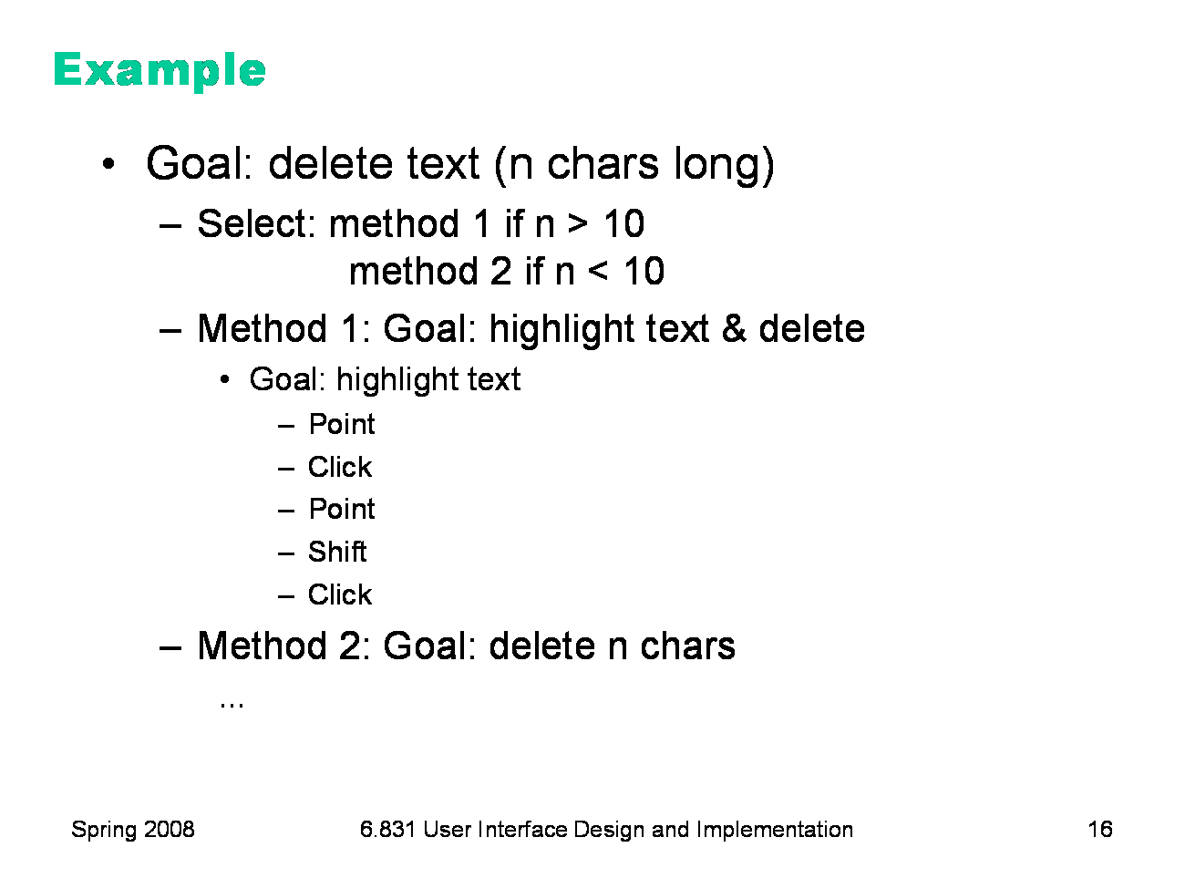
Here’s an outline of a GOMS model for the text-deletion example we’ve been using.  Notice the selection rule that chooses between two methods for achieving the goal, based on an observation of how many characters need to be deleted.

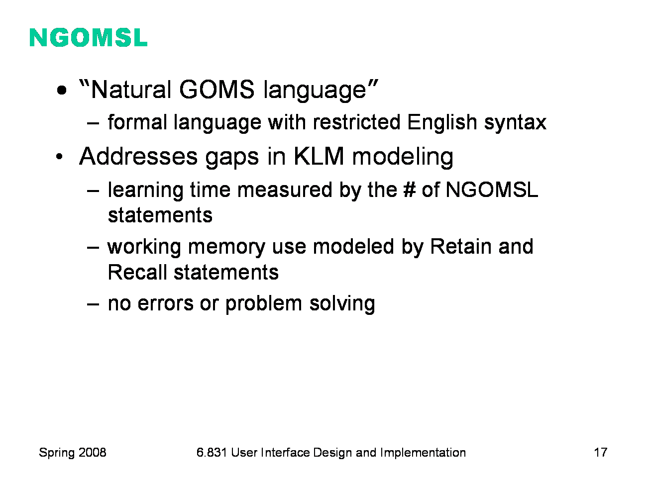
GOMS has several variants.  One of them, called NGOMSL, uses a formal language to restrict how you model goals, subgoals, and selection rules.  The benefit of the formal language is that each statement roughly corresponds to a primitive mental chunk, so you can estimate the learning time of a task by simply counting the number of statements in the model for the task.  The language also has statements that represent working memory operations (Retain and Recall), so that excessive use of working memory can be estimated by executing the model.

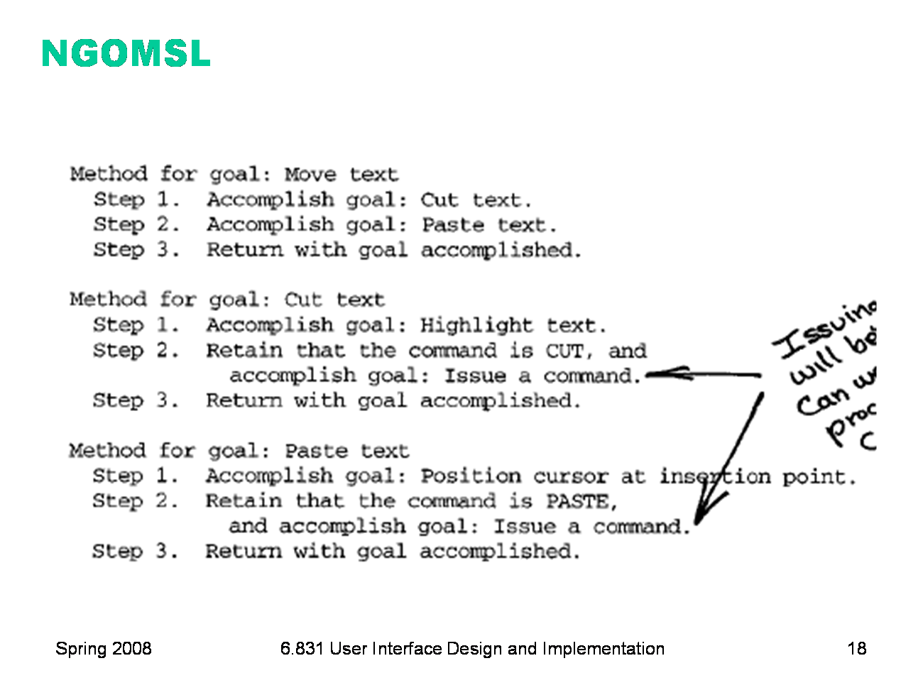
Here’s a snippet of an NGOMSL model for text editing (from John & Kieras, “The GOMS Family of User Interface Analysis Techniques: Comparison and Contrast”, ACM TOCHI, v3 n4, Dec 1996).

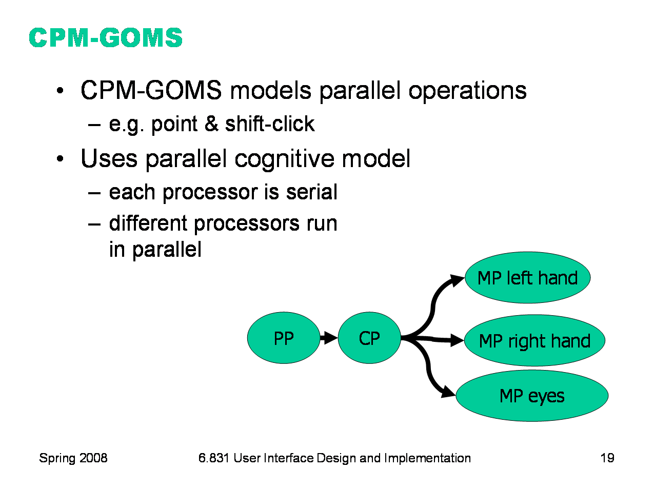
CPM-GOMS (Cognitive-Motor-Perceptual) is another variant of GOMS, which is even more detailed than the keystroke-level model.  It tackles the serial assumption of KLM, allowing multiple operators to run at the same time.  The parallelism is dictated by a model very similar to the Card/Newell/Moran information processing model we saw earlier.  We have a perceptual processor (PP), a cognitive processor (CP), and multiple motor processors (MP), one for each major muscle system that can act independently.  For GUI interfaces, the muscles we mainly care about are the two hands and the eyes.

The model makes the simple assumption that each processor runs tasks serially (one at a time), but different processors run in parallel.

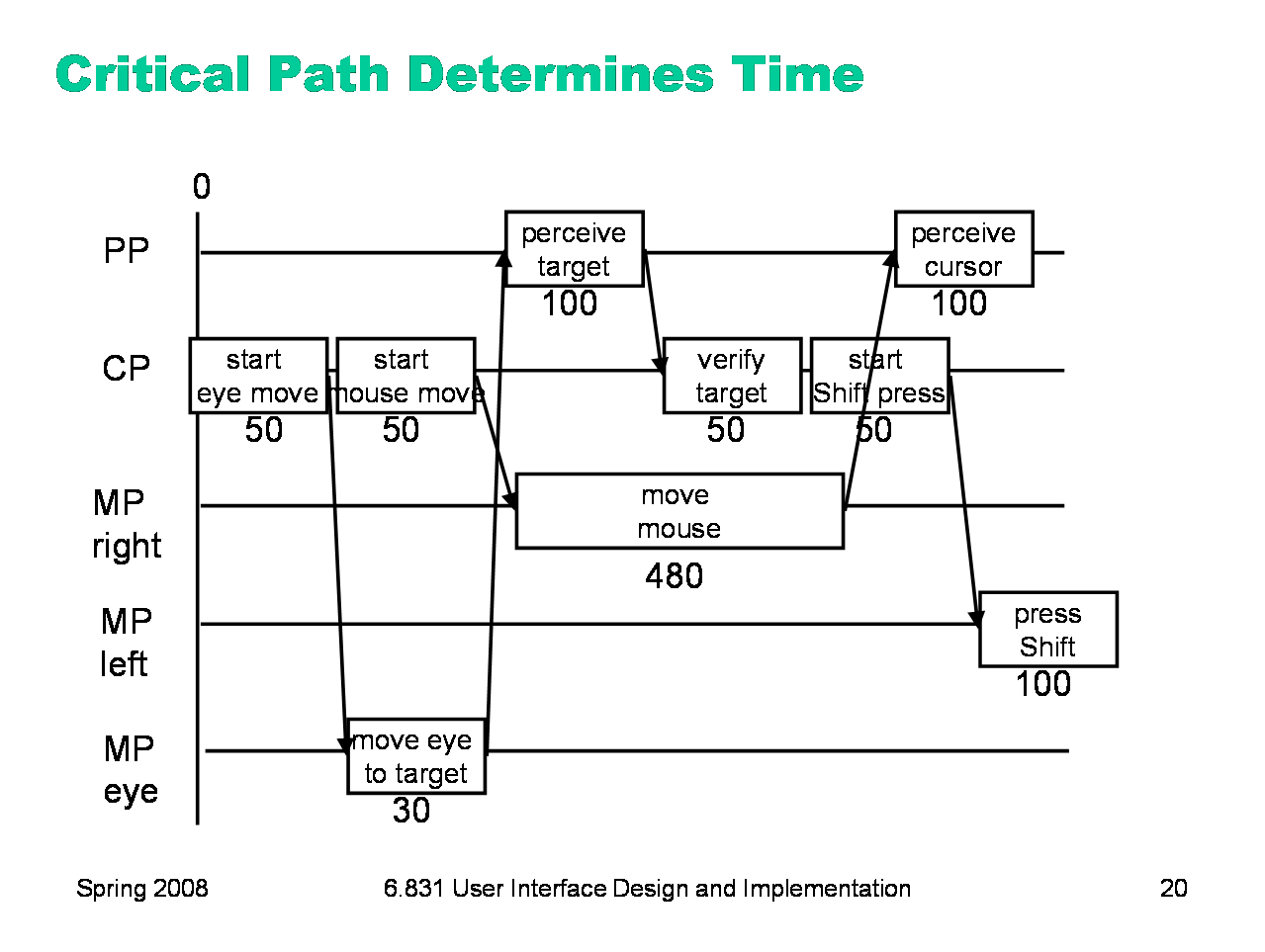
We build a CPM-GOMS model as a graph of tasks.  Here’s the start of a Point-Shift-click operation.

First, the cognitive processor (which initiates everything) decides to move your eyes to the pointing target, so that you’ll be able to tell when the mouse pointer reaches it.

Next, the eyes actually move (MP eye), but in parallel with that, the cognitive processor is deciding to move the mouse.  The right hand’s motor processor handles this, in time determined by Fitts’s Law.

While the hand is moving, the perceptual processor and cognitive processor are perceiving and deciding that the eyes have found the target.

Then the cognitive processor decides to press the Shift key, and passes this instruction on to the left hand’s motor processor.

In CPM-GOMS, what matters is the critical path through this graph of overlapping tasks — the path that takes the longest time, since it will determine the total time for the method.

Notice how much more detailed this model is!  This would be just P K in the KLM model.  With greater accuracy comes a lot more work.

Another issue with CPM-GOMS is that it models extreme expert performance, where the user is working at or near the limits of human information processing speed, parallelizing as much as possible, and yet making no errors.

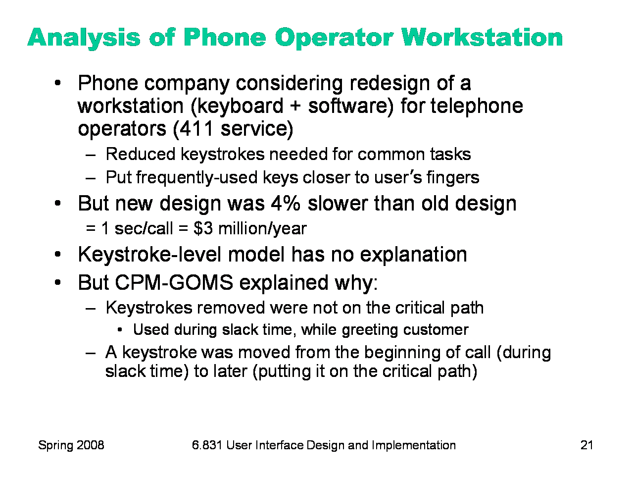
CPM-GOMS had a real-world success story.  NYNEX (a phone company) was considering replacing the workstations of its telephone operators.  The redesigned workstation they were thinking about buying had different software and a different keyboard layout.  It reduced the number of keystrokes needed to handle a typical call, and the keyboard was carefully designed to reduce travel time between keys for frequent key sequences.  It even had four times the bandwidth of the old workstation (1200 bps instead of 300).  A back-of-the-envelope calculation, essentially using the KLM model, suggested that it should be 20% faster to handle a call using the redesigned workstation.  Considering NYNEX’s high call volume, this translated into real money — every second saved on a 30-second operator call would reduce NYNEX’s labor costs by $3 million/year.

But when NYNEX did a field trial of the new workstation (an expensive procedure which required retraining some operators, deploying the workstation, and using the new workstation to field calls), they found it was actually 4% slower than the old one.

A CPM-GOMS model explained why.  Every operator call started with some “slack time”, when the operator greeted the caller (e.g. “Thank you for calling NYNEX, how can I help you?”)  Expert operators were using this slack time to set up for the call, pressing keys and hovering over others.  So even though the new design removed keystrokes from the call, the removed keystrokes occurred during the slack time — not on the critical path of the call, after the greeting.  And the 4% slowdown was due to moving a keystroke out of the slack time and putting it later in the call, adding to the critical path.  On the basis of this analysis, NYNEX decided not to buy the new workstation.  (Gray, John, & Atwood, “Project Ernestine: Validating a GOMS Analysis for Predicting and Explaining Real-World Task Performance”, Human-Computer Interaction, v8 n3, 1993.)

This example shows how predictive evaluation can explain usability problems, rather than merely identifying them (as the field study did).