September 12, 2005
Splay trees are binary search trees with good balance properties when amortized over a sequence of operations. It does not require extra marking fields, like the color field in the red-black tree.
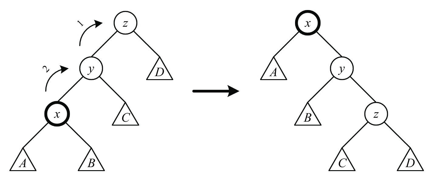
When a node \(x\) is accessed, we perform a sequence of splay steps to move \(x\) to the root of the tree. There are 6 types of splay steps, each consisting of 1 or 2 rotations (see Figures 1, 2, and 3).
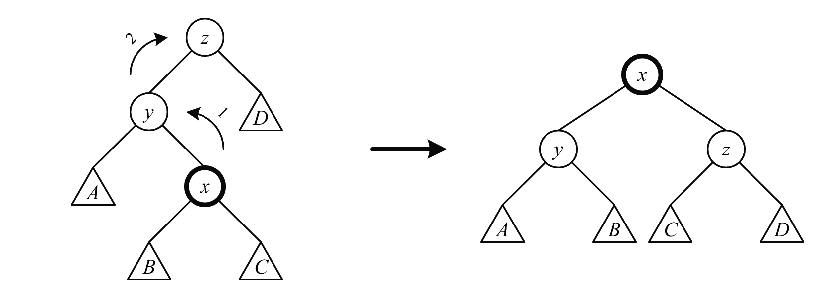
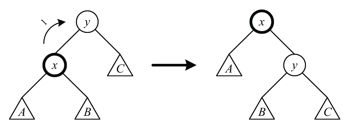
We perform splay steps to \(x\) (\(rr\), \(ll\), \(lr\), or \(rl\), depending on whether \(x\) and \(x\)’s parent are left or right children) until \(x\) is either the root or a child of the root. In the latter case, we need to perform either a \(r\) or \(l\) splay step to make \(x\) the root. This completes a splay of \(x\).
One intuition behind this is that the most recently used node is now moved to the root, and therefore this will speed up further queries to this node. Another, and arguably more important intuition is that, it also helps further queries to other nodes, because a splay operation will move up the nodes that are deep in the tree, as we will see in the next subsection. In general, the cost of performing this operation will be absorbed by the potential of a node, which measures the ’fatness’ of a node.
We will show that splay operations have amortized cost \(O(\log n)\), and that consequently all splay tree operations have amortized cost \(O(\log n)\).
For amortized analysis, we define the following for each node \(x\):
a constant weight \(w(x) > 0\) (for the analysis, this can be arbitrary)
weight sum \(s(x) = \sum_{y \in \textrm{subtree}(x)} w(y)\) (where \(\textrm{subtree}(x)\) is the subtree rooted at \(x\), including \(x\))
rank \(r(x) = \log s(x)\)
We use \(r(x)\) as the potential of a node. The potential function after \(i\) operations is thus \(\phi(i) = \sum_{x \in \textrm{tree}} r(x)\).
Lemma: The amortized cost of a splay step on node \(x\) is \(\le 3(r'(x) - r(x)) + 1\), where \(r\) is rank before the splay step and \(r'\) is rank after the splay step. Furthermore, the amortized cost of the \(rr\), \(ll\), \(lr\), and \(rl\) splay steps is \(\le 3(r'(x) - r(x))\).
Proof. We will consider only the \(rr\) splay step (refer to Figure 1). The actual cost of the splay step is 2 (for 2 rotations). The splay step only affects the potentials/ranks of nodes \(x\), \(y\), and \(z\); we observe that \(r'(x) = r(z)\), \(r(y) \ge r(x)\), and \(r'(y) \le r'(x)\).
The amortized cost of the splay step is thus: \[\begin{aligned} \textrm{amortized cost} & = 2 + \phi(i + 1) - \phi(i) \\ & = 2 + (r'(x) + r'(y) + r'(z)) - (r(x) + r(y) - r(z)) \\ & = 2 + (r'(x) - r(z)) + r'(y) + r'(z) - r(x) - r(y) \\ & \le 2 + 0 + r'(x) + r'(z) - r(x) - r(x) \\ & = 2 + r'(x) + r'(z) - 2r(x)\end{aligned}\]
The log function is concave, i.e., \(\frac{\log a + \log b}{2} \le \log\left(\frac{a + b}{2}\right)\). Thus we also have (\(s\) is weight sum before the splay step and \(s'\) is weight sum after the splay step): \[\begin{aligned} \frac{\log(s(x)) + \log(s'(z))}{2} & \le \log\left(\frac{s(x) + s'(z)}{2}\right) \\ \frac{r(x) + r'(z)}{2} & \le \log\left(\frac{s(x) + s'(z)}{2}\right) \textrm{(note that $s(x) + s'(z) \le s'(x)$)}\\ & \le \log\left(\frac{s'(x)}{2}\right) \\ & = r'(x) - 1 \\ r'(z) & \le 2r'(x) - r(x) - 2\end{aligned}\]
Thus the amortized cost of the \(rr\) splay step is \(\le 3(r'(x) - r(x))\).
The same inequality must hold for the \(ll\) splay step; the inequality also holds for the \(lr\) (and \(rl\)) splay steps. The \(+ 1\) in the lemma applies for the \(r\) and \(l\) cases. ◻
Corollary: The amortized cost of a splay operation on node \(x\) is \(O(\log n)\).
Proof. The amortized cost of a splay operation on \(x\) is the sum of the amortized costs of the splay steps on \(x\) involved: \[\begin{aligned} \textrm{amortized cost} & = \sum_{i} \textrm{cost}(\textrm{splay\_step}_{i}) \\ & \le \sum_{i} \left(3r^{i + 1}(x) - r^{i}(x)\right) + 1 \\ & = 3(r(\textrm{root}) - r(x)) + 1\end{aligned}\]
The \(+ 1\) comes from the last \(r\) or \(l\) splay step (if necessary). If we set \(w(x) = 1\) for all nodes in the tree, then \(r(\textrm{root}) = \log n\) and we have: \[\textrm{amortized cost} \le 3\log n + 1 = O(\log n)\] ◻
There are more applications mentioned in class, about how to more cleverly set the initial weight \(w_i\)’s. Please refer to the raw notes.
For the find operation, we perform a normal BST find followed by a splay operation on the node found (or the leaf node last encountered, if the key was not found). We can charge the cost of going down the tree to the splay operation. Thus the amortized cost of find is \(O(\log n)\).
For the insert operation, we perform a normal BST insert followed by a splay operation on the node inserted. Assume node \(x\) is inserted at depth \(k\). Denote the parent of \(x\) as \(y_{1}\), \(y_{1}\)’s parent as \(y_{2}\), and so on (the root of the tree is \(y_{k}\)). Then the change in potential due to the insertion of \(x\) is (\(r\) is rank before the insertion and \(r'\) is rank after the insertion, \(s\) is weight sum before the insertion): \[\begin{aligned} \Delta\phi & = \sum_{j = 1}^{k} \left(r'(y_{j}) - r(y_{j})\right) \\ & = \sum_{j = 1}^{k} \left(\log(s(y_{j}) + 1) - \log(s(y_{j})\right) \\ & = \sum_{j = 1}^{k} \log\left(\frac{s(y_{j}) + 1}{s(y_{j})}\right) \\ & = \log\left(\prod_{j = 1}^{k} \frac{s(y_{j}) + 1}{s(y_{j})}\right) \textrm{(note that $s(y_{j}) + 1 \le s(y_{j + 1})$)} \\ & \le \log\left(\frac{s(y_{2})}{s(y_{1})} \cdot \frac{s(y_{3})}{s(y_{2})} \cdots \frac{s(y_{k})}{s(y_{k - 1})} \cdot \frac{s(y_{k}) + 1}{s(y_{k})}\right) \\ & = \log\left(\frac{s(y_{k}) + 1}{s(y_{1})}\right) \\ & \le \log n\end{aligned}\]
The amortized cost of the splay operation is also \(O(\log n)\), and thus the amortized cost of insert is \(O(\log n)\).
We have proved the following:
Theorem: All splay tree operations have amortized cost \(O(\log n)\).