October 27, 2006
\(NP\)-hard problems are a vast family of problems that, to the best of our knowledge, cannot be solved in polynomial time.1 When presented with a \(NP\)-hard problem, we can take one of three possible strategies:
Run a super-polynomial algorithm anyway. Techniques such as branch-and-bound (known as \(A^*\) search in the AI world) allow us to enumerate options in a way such that we can ignore most of the problem space. However, the desired complexity bounds of these algorithms are usually not provable, and even “slightly” super-polynomial is often too much to be practical.
Assume that the input is random, and find an algorithm that will perform well in the average case. For example, the maximum clique problem, which is \(NP\)-hard, can actually be solved efficiently assuming a random input because the maximum clique in a randomly chosen graph is small. This assumption is often used in practice, but the problem is that not everyone will agree on whether the input distribution is random.
Settle for a suboptimal solution (an approximation) that can be found in polynomial time, and prove that this solution is “good enough”. This is the technique that we will look at in the rest of the lecture.
Definition: An optimization problem consists of:
A set of instances \(I\)
A set of solutions \(S(I)\)
An objective function2 \(f: S(I)\to \mathbb{R}\)
The problem is to find \(s\in S(I)\) that maximizes (or minimizes) \(f(s)\).
Example:
Graph Coloring is an optimization problem with the following form:
\(I\): graphs
\(S(I)\): assignments of colors to each vertex such that no neighbors have the same color
\(f(s)\): number of colors used in \(s\)
Thus, given a graph, we want to find the minimum number of colors we can use to color the vertices such that no two adjacent vertices have the same color.
Some technicalities: When analyzing the complexity of optimization problems, we will assume that all inputs and ranges of \(f\) are rational numbers. We will also assume that if \(\sigma\) is an optimal solution, then \(f(\sigma)\) is polynomial in the number of bits in the input. Our goal will be to find algorithms that have a runtime polynomial in the representation of the input in bits.
Often, when people refer to \(NP\)-hard problems, they are referring to decision problems, which are algorithms for which the output is yes or no. For example, a decision version of the Graph Coloring problem is determining whether or not a graph is 3-colorable. We need a notion of \(NP\)-hardness that applies to optimization problems as well.
Definition (NP-hardness): An optimization problem is \(NP\)-hard if it can be used as a subroutine to solve an \(NP\)-hard decision problem in polynomial time, with the optimization problem used as a black box.
Definition: An approximation algorithm is any algorithm that gives a feasible solution to an optimization problem.
The above definition of an approximation algorithm gives no measure of how good the algorithm actually is. For instance, a valid approximation algorithm for the Graph Coloring problem is to color each vertex with its own color. Thus, we need a way to differentiate approximation algorithms based on how “good” they actually are. In the rest of this lecture, we discuss two ways to measure the “goodness” of an algorithm by comparing its output to the optimal solution.
One way to compare the output of an approximation algorithm to the optimal solution is to take the absolute difference between them. If we can bound this difference to a constant for any input, then we have an absolute approximation algoirthm.
Definition: \(A\) is a \(k\)-absolute approximation algorithm if \(|A(I) - OPT(I)| \le k\).
The absolute value in the above definition allows us to cover both maximization and minimization problems with the same definition - \(A(I) \le OPT(I)\) in a maximization problem, and \(A(I)\ge OPT(I)\) in a minimization problem.
Our next example will involve planar graphs. Recall the following definition:
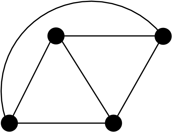
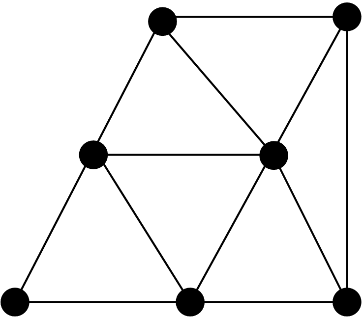
Definition: A planar graph is a graph that can be drawn on the blackboard without any edges crossing.
Figure 1. Examples of graphs that are planar:
|
|
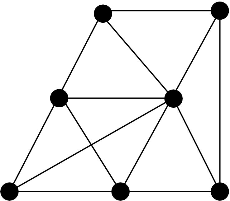
Figure 2. Example of a graph that is not planar:
 |
Euler’s formula for planar graphs tells us that \(m \le 3n-6\) for \(n\ge 3\), where \(n\) is the number of vertices and \(m\) is the number of edges. As a particular corollary, every planar graph has at least one vertex with degree less than 6, since the sum of the degrees of the vertices is \(2m\), which by Euler’s formula is less than \(6n\).
Definition: Planar Graph Coloring is a restricted version of Graph Coloring where the inputs are constrained to be planar.
Theorem: There exists a 1-absolute approximation algorithm for Planar Graph Coloring.
Proof. We will exhibit such an algorithm. First, note that if a graph is 1-colorable, then it has no edges and we can trivially color it. Similarly, a 2-colorable graph is bipartite, and all other graphs require at least 3 colors. We can color any other planar graph with 4 colors by the famous Four Color Theorem.
The complete algorithm for an arbitrary planar graph thus works as follows:
If the graph is 1-colorable, then color it optimally.
If the graph is bipartite, color it with 2 colors.
Otherwise, the graph requires at least 3 colors. Color it with 4 colors using the Four Color Theorem.
This algorithm achieves a 1-absolute approximation. ◻
Unfortunately, the set of \(NP\)-hard problems with absolute approximations is very small. This is because in general, we can transform an absolute approximation into an exact solution by a scaling technique, which would imply that \(P=NP\). Assuming that \(P\ne NP\), we can prove that no absolute approximation exists for problems that have this property. We will do this for Knapsack, one of the first problems that was shown to be \(NP\)-complete, and for Maximum Independent Set, another \(NP\)-complete problem.
Definition: In the Knapsack problem, we are given a knapsack of size \(B\) and items \(i\) with size \(s_i\) and profit \(p_i\). We can think of this as a kind of shoplifting problem; the goal is to find the subset of the items with maximum total profit that fits into the knapsack.
Theorem: There is no \(k\)-absolute approximation algorithm for Knapsack for any number \(k\).
Proof. Suppose for the sake of contradiction that we have a \(k\)-absolute approximation algorithm. First we will consider the case where the prices \(p_i\) are integers. We multiply all the prices by \(k+1\) and run our \(k\)-absolute approximation algorithm on the resulting instance. The difference between any two solutions in the original instance is at least 1, so the difference between any two solutions in the scaled instance is at least \(k+1\). As a result of scaling, the optimum solution increases by a factor of \(k+1\), but our \(k\)-approximate solution is within \(k\) of this. Therefore, the approximation algorithm gives an exact solution for the scaled graph. We divide by \(k+1\) to obtain an optimal solution for the original graph. This would constitute a polynomial-time solution for a problem that is believed to be super-polynomial, so we have a contradiction.
Note that if the prices are rational numbers rather than integers, we can simply multiply all of the prices by their common denominator, which has a polynomial number of bits. Then the problem reduces to the integer case above. ◻
Definition: In the Maximum Independent Set problem, we are given a graph \(G\) and we must find the largest subset of the vertices in \(G\) such that there is no edge between any two vertices in the set.
Note that a graph’s maximum independent set is identical to the maximum clique in the complementary graph. (The complement of a graph is the graph obtained by taking the same set of vertices as in the original graph, and placing edges only between vertices that had no edges between them in the original graph.)
Theorem: There is no \(k\)-absolute approximation for Maximum Independent Set, for any number \(k\).
Proof. Suppose for the sake of contradiction that we have a \(k\)-absolute approximation algorithm for Maximum Independent Set. Although there are no numbers to scale up in this problem, there is still a scaling trick we can use.
For an instance \(G\), we make a new instance \(G'\) out of \(k+1\) copies of \(G\) that are not connected to each other. Then a maximum independent set in \(G'\) is composed of one independent set in each copy of \(G\), and in particular, \(OPT(G')\) is \(k+1\) times as large as \(OPT(G)\). A \(k\)-absolute approximation to a maximum independent set of \(G'\) has size at least \((k+1)|OPT(G)|-k\). This approximation consists of independent sets in each copy of \(G\). At least one of the copies must contain a maximum independent set (i.e., an independent set of size \(|OPT(G)|\)), because otherwise the total number of elements in the approximation would be at most \((k+1)|OPT(G)| - (k+1)\), contradicting the assumption that we have a \(k\)-absolute approximation. Hence, we can obtain an exact solution to Maximum Independent Set in polynomial time, which we presume is impossible. ◻
Since absolute approximations are often not achievable, we need a new technique—a new way to measure approximations. Since we can’t handle additive factors, we will try multiplicative ones.
Definition: An \(\alpha\)-approximate solution \(S(I)\) has value \(\le \alpha|OPT(I)|\) if the problem is a minimization problem and value \(\ge |OPT(I)|/\alpha\) if the problem is a maximization problem.
Definition: An algorithm has an approximation ratio \(\alpha\) if it always yields an \(\alpha\)-approximate solution.
Of course, \(\alpha\) must be at least 1 in order for these definitions to make sense. We often call an algorithm with an approximation ratio \(\alpha\) an \(\alpha\)-approximate algorithm. Since absolute approximations are so rare, people will assume that a relative approximation is intended when you say this.
Once we have formulated an algorithm, how can we prove that it is \(\alpha\)-approximate? In general, it is hard to describe the optimal solution, since it is our inability to talk about \(OPT\) that prevents us from formulating an exact polynomial-time algorithm for the problem. Nevertheless, we can establish that an algorithm is \(\alpha\)-approximate by comparing its output to some upper or lower bound on the optimal solution.
Greedy approximation algorithms often wind up providing relative approximations. These greedy methods are algorithms in which we take the best local step in each iteration and hope that we don’t accumulate too much error by the time we are finished.
To illustrate the design and analysis of an \(\alpha\)-approximation algorithm, let us consider the Parallel Machine Scheduling problem, a generic form of load balancing.
Parallel Machine Scheduling:
Given \(m\) machines \(m_i\) and \(n\) jobs with processing times \(p_j\), assign the jobs to the machines to minimize the load
\[\max\limits_{i} \sum\limits_{j \in i} p_j,\]
the time required for all machines to complete their assigned jobs. In scheduling notation, this problem is described as \(\mathrm {P \parallel C_{\max}}\).
A natural way to solve this problem is to use a greedy algorithm called list scheduling.
Definition: A list scheduling algorithm assigns jobs to machines by assigning each job to the least loaded machine.
Note that the order in which the jobs are processed is not specified.
To analyze the performance of list scheduling, we must somehow compare its solution for each instance \(I\) (call this solution \(A(I)\)) to the optimum \(OPT(I)\). But we do not know how to obtain an analytical expression for \(OPT(I)\). Nonetheless, if we can find a meaningful lower bound \(LB(I)\) for \(OPT(I)\) and can prove that \(A(I) \le \alpha \cdot LB(I)\) for some \(\alpha\), we then have
\[\begin{array}{lcl} A(I) & \le & \alpha \cdot LB(I) \\ & \le & \alpha \cdot OPT(I). \end{array}\]
Using the idea of lower-bounding \(OPT(I)\), we can now determine the performance of list scheduling.
Claim: List scheduling is a \((2-1/m)\)-approximation algorithm for Parallel Machine Scheduling.
Proof. Consider the following two lower bounds for the optimum load \(OPT(I)\):
the maximum processing time \(p = \max_j p_j,\)
the average load \(L = \sum_j p_j/m.\)
The maximum processing time \(p\) is clearly a lower bound, as the machine to which the corresponding job is assigned requires at least time \(p\) to complete its tasks. To see that the average load is a lower bound, note that if all of the machines could complete their assigned tasks in less than time \(L\), the maximum load would be less than the average, which is a contradiction. Now suppose machine \(m_i\) has the maximum runtime \(L = c_{\max}\), and let job \(j\) be the last job that was assigned to \(m_i\). At the time job \(j\) was assigned, \(m_i\) must have had the minimum load (call it \(L_i\)), since list scheduling assigns each job to the least loaded machine. Thus,
\[\begin{array}{lcl} \sum\limits_{\mbox{all machine i}} p_i & \ge & m L_i + p_j \\ & = & m (L - p_j) + p_j \end{array}\]
Therefore,
\[\begin{array} {lcl} OPT(I) & \ge & \frac{1}{m} \left( m (L - p_j) + p_j \right) \\ & = & L - (1-1/m) p_j, \\ \mbox{so} \\ L & \le & OPT(I) + (1 - 1/m) p_j \\ & \le & OPT(I) + (1 - 1/m) OPT(I) \\ & \le & (2 - 1/m) OPT(I). \end{array}\]
The solution returned by list scheduling is \(c_{\max}\), and thus list scheduling is a \((2-1/m)\)-approximation algorithm for Parallel Machine Scheduling.
The example with \(m(m-1)\) jobs of size \(1\) and one job of size \(m\) for \(m\) machines shows that we cannot do better than \((2-1/m)OPT(I)\). ◻
Definition: In the Maximum Cut problem (for undirected graphs), we are given an undirected graph and wish to partition the vertices into two sets such that the number of edges crossing the partition is maximized.
Example (A Greedy Algorithm for Maximum Cut): In each step, we pick any vertex and place it on one side of the cut or the other. In particular, we place each vertex on the side opposite most of its previously placed neighbors. (If the vertex has no previously placed neighbors, or an equal number of neighbors on each side, then we place it on either side.) The algorithm terminates when all vertices have been placed.
We can say very little about the structure of the optimum solution to Maximum Cut for an arbitrary graph, but there’s an obvious bound on the number of edges in the cut, namely \(m\), the total number of edges in the graph. We can measure the goodness of our greedy algorithm’s approximation with respect to this bound.
Theorem: The aforementioned greedy algorithm for Maximum Cut is 2-approximate.
Proof. We say that an edge is “fixed” if both of its endpoints have been placed. Every time we place a vertex, some number of edges get fixed. At least half of these edges are cut by virtue of the heuristic used to choose a side for the vertex. The algorithm completes when all edges have been fixed, at which point \(m/2\) edges have been cut, whereas we know that optimum solution has at most \(m\) edges. ◻
The approach we just described was the best known approximation algorithm for Maximum Cut for a long time. It was improved upon in the last decade using a technique that we will discuss in the next lecture.
Example A Clustering Problem: Suppose we are given a set of points, along with distances satisfying the triangle inequality. Our goal is to partition the points into \(k\) groups such that the maximum diameter of the groups is minimized. The diameter of a group is defined to be the maximum distance between any two points in the group.
An approximation algorithm for this problem involves first picking \(k\) cluster “centers” greedily. That is, we repeatedly pick the point at the greatest distance from the existing centers to be a new center. Then we assign the remaining points to the closest centers. The analysis of this problem is left as a problem set exercise.
As we demonstrated, Maximum Cut has a constant-factor approximation. We will now consider an algorithm that has no constant-factor approximation, i.e., \(\alpha\) depends on the size of the input.
Definition: In the Set Cover problem, we are given a collection of \(n\) items and a collection of (possibly overlapping) sets, each of which contains some of the items. A cover is a collection of sets whose union contains all of the items. Our goal is to produce a cover using the minimum number of sets.
A natural local step for Set Cover is to add a new set to the cover. An obvious greedy strategy is to always choose the set that covers the most new items.
Theorem: A greedy algorithm for Set Cover that always chooses the set that covers the most new items is \(O(\log n)\)-approximate.
Proof. Suppose that the optimum cover has \(k\) sets. Then at a stage where \(r\) items remain to be covered, some set covers \(r/k\) of them. Therefore, choosing the set that covers the most new points reduces the number of uncovered points to \(r-r/k = r(1-1/k)\). If we start with \(n\) points and repeat this process \(j\) times, \(r\le n(1-1/k)^j\). Since \(r\) is an integer, we are done when \(n(1-1/k)^j < 1\). This happens when \(j = O(k\log n)\). Hence, \(\alpha = j/k = O(\log n)\). ◻
This result is much better than an \(O(n)\)-approximate solution, but you have to wonder if we could do better with a cleverer algorithm. People spent a long time trying to find a constant approximation. Unfortunately, it was recently proven that \(O(\log n)\) is the best possible polynomial-time approximation.
However, we can do better for a special case of Set Cover called Vertex Cover. Both problems are \(NP\)-hard, but it turns out that the latter does indeed have a constant factor approximation.
Definition: In the Vertex Cover problem, we are given a graph \(G\), and we wish to find a minimal set of vertices containing at least one endpoint of each edge.
After seeing a greedy algorithm for Set Cover, it might seem natural to devise a scheme for Vertex Cover in which a local step consists of picking the vertex with the highest uncovered indegree. This does indeed give a \(O(\log n)\) approximation, but we can do better with another heuristic.
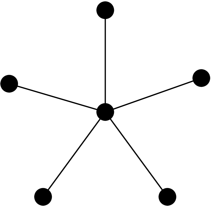
As a starting point, imagine that instead of looking at the number of covered edges on each vertex, we simply picked any uncovered edge and covered it. Clearly one of the two endpoints for the edge is in the optimum cover. Unfortunately, we might get unlucky and pick the wrong one. Consider the graph in Figure 1. If we chose the peripheral vertices first, our cover would contain \(n-1\) vertices.
To solve this problem, when we choose an edge to cover, we add both of its endpoints to the cover. This gives us a 2-approximate cover because one of the two endpoints is in the optimum cover. This is a beautiful case of bounding an approximation against a bound of the optimum solution without actually knowing the optimum solution.
Relatively recently, someone improved the vertex cover bound to a \(2-O(\log\log n/\log n)\) approximation with a significant amount of work. It is known to be impossible to do better than \(4/3\), but nobody knows how to close the gap.
The obvious question to ask now is how good an \(\alpha\) we can obtain.
Definition: A polynomial approximation scheme (PAS) is a set of algorithms \(\{ A_\varepsilon \}\) for which each \(A_\varepsilon\) is a polynomial-time \((1+\varepsilon)\)-approximation algorithm.
Thus, given any \(\varepsilon >0\), a PAS provides an algorithm that achieves a \((1+\varepsilon)\)-approximation. In order to devise a PAS we can use a method called \(k\)-enumeration.
Definition: An approximation algorithm using \(k\)-enumeration finds an optimal solution for the \(k\) most important elements in the problem and then uses an approximate polynomial-time method to solve the reminder of the problem.
We can do the following:
Enumerate all possible assignments of the \(k\) largest jobs.
For each of these partial assignments, list schedule the remaining jobs.
Return as the solution the assignment with the minimum load.
Note that in enumerating all possible assignments of the \(k\) largest jobs, the algorithm will always find the optimal assignment for these jobs. The following claim demonstrates that this algorithm provides us with a PAS.
Claim: For any fixed \(m\), \(k\)-enumeration yields a polynomial approximation scheme for Parallel Machine Scheduling.
Proof. Let us consider the machine \(m_i\) with maximum runtime \(c_{\max}\) and the last job that \(m_i\) was assigned.
If this job is among the \(k\) largest, then it is scheduled optimally, and \(c_{\max}\) equals \(OPT(I)\).
If this job is not among the \(k\) largest, without loss of generality we may assume that it is the \((k+1)\)th largest job with processing time \(p_{k+1}\). Therefore, \[%\begin{array} {lcl} A(I) \le OPT(I) + p_{k+1}.\] Suppose otherwise, \(A(I) > OPT(I) + p_{k+1}\). Remember we must have scheduled the last job to the machine with the least load, that implies all machines had load greater than \(OPT(I)\). But we argued before than \(nOPT(I) \geq \Sigma p_i\), the sum of all processing times. So, before we scheduled all jobs, the total time is already larger than the sum of all the processing times, contradiction.
However, \(OPT(I)\) can be bound from below in the following way: \[OPT(I) \ge \frac{k p_k}{m},\]
because \(\frac{k p_k}{m}\) is the minimum average load when the largest \(k\) jobs have been scheduled.
Now we have: \[\begin{array} {lcl} A(I) & \le & OPT(I) + p_{k+1} \\ & \le & OPT(I) + OPT(I) \frac{m}{k} \\ & = & OPT(I) \left( 1+\frac{m}{k} \right). \end{array}\]
Given \(\varepsilon > 0\), if we let \(k\) equal \(m/\varepsilon\), we will get \[c_{\max} \le (1+\varepsilon) OPT(I).\]
Finally, to determine the running time of the algorithm, note that because each of the \(k\) largest jobs can be assigned to any of the \(m\) machines, there are \(m^k = m^{m/\varepsilon}\) possible assignments of these jobs. Since the list scheduling performed for each of these assignments takes \(O(n)\) time, the total running time is \(O(nm^{m/\epsilon})\), which is polynomial because \(m\) is fixed. Thus, given an \(\varepsilon >0\), the algorithm is a \((1+\varepsilon)\)-approximation, and so we have a polynomial approximation scheme. ◻
Consider the PAS in the previous section for \({\rm P \parallel C_{\max}}\). The running time for the algorithm is prohibitive even for moderate values of \(\varepsilon\). The next level of improvement, therefore, would be approximation algorithms that run in time polynomial in \(1/ \varepsilon\), leading to the definition below.
Definition: Fully Polynomial Approximation Scheme (FPAS) is a set of approximation algorithms such that each algorithm \(A(\varepsilon)\) in this set runs in time that is polynomial in the size of the input, as well as in \(1/ \varepsilon\).
There are few \(NP\)-complete problems that allow for FPAS. Below we discuss FPAS for the Knapsack problem.
The Knapsack problem receives as input an instance \(I\) of \(n\) items with profits \(p_i\), sizes \(s_i\) and knapsack size (or capacity) \(B\). The output of the Knapsack problem is the subset \(S\) of items of total size at most \(B\), and that has profit:
\[\max \sum\limits_{i \in S} p_i.\]
Suppose now that the profits are integers; then we can write a \(DP\) algorithm based on the minimum size subset with profit \(p\) for items \(1, \, 2, \, \ldots, \, r\) as follows:
\[M(r,p) = \min \left\{ M(r-1,p), M(r-1, p-p_r) + s_r \right\}.\]
The corresponding table of values can be filled in \(O\left(n \sum_i p_i \right)\) (note that this is not a FPAS in itself).
Now, we consider the general case where the profits are not assumed to be integers. Once again, we use a rounding technique but one that can be considered a generic approach for developing FPAS for other \(NP\)-complete problems that allows for FPAS. Suppose we multiplied all profits \(p_i\) by \(n/(\varepsilon \cdot OPT)\); then the new optimal objective value is apparently \(n/\varepsilon\). Now, we can round the profits down to the nearest integer, and hence the optimal objective value decreases at most by \(n\); expressed differently, the decrease in objective value is at most \(\varepsilon \cdot OPT\). Using the \(DP\) algorithm above, we can therefore find the optimal solution to the rounded problem in \(O(n^2/ \varepsilon)\) time, thus providing us with a FPAS in \(1/\varepsilon\).
Briefly, \(P\) is the set of problems solvable in polynomial time, and \(NP\) is a particular superset of \(P\). A problem is \(NP\)-hard if it is at least as hard as all problems in \(NP\), and \(NP\)-complete if it is in \(NP\) and it is also \(NP\)-hard. An unproven but generally accepted conjecture, which we will assume is true, is that \(P\ne NP\).↩︎
The restriction that the range of the objective function is \(R\) might be limiting in some situations, but most problems can be formulated this way.↩︎