Homework 2: Parallel Sparse Conjugate Gradients
Due date: 04/14/2005 by 11:59 PM
Notes:
- Submit your solutions as before (see instructions for Homeworks 0 or 1). Compile all your conclusions and timing information for both parts into one single PDF or PS document.
- If you consented to the productivity survey:
- Make sure you run the following script before beginning work on
the problem set: /home/lorin/inst/sensors/setup.sh
- If your last name begins with A through M, attempt the MPI question first;
otherwise attempt the Star-P question first
- For the Star-P question, please save your session and timing information in a diary (use diary on or diary filename) and submit it along with your solutions.
- Last, but not the least, please complete the activity logs!
- More notes and hints to follow ...
In this problem set, you will implement a parallel iterative solver for solving a linear system of equations of the form
 |
(1) |
where
 is
sparse, symmetric and positive definite and
is
sparse, symmetric and positive definite and
 .
.
The matrix must be stored using either the compressed row or
compressed column formats discussed in the class. Further, in
a distributed memory setting, the matrix will be row distributed and
you may assume that each process has the same number of rows ( ).
).
Let  be the number of non-zero entries of
 . Then
can be stored in the compressed sparse row format using
three arrays, vals, cols and rows as
follows: vals
. Then
can be stored in the compressed sparse row format using
three arrays, vals, cols and rows as
follows: vals
 stores the non-zero
entries in
stores the non-zero
entries in  in row-major order; cols
stores the column numbers for the non-zero entries
for each row; rows
in row-major order; cols
stores the column numbers for the non-zero entries
for each row; rows
 stores the
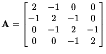
cumulative number of non-zero entries in each row. For example, if
then vals = {2, -1, -1, 2, -1, -1, 2, -1, -1, 2},
cols = {0, 1, 0, 1, 2, 1, 2, 3, 2, 3} and rows =
{0, 2, 5, 8, 10}.
stores the
cumulative number of non-zero entries in each row. For example, if
then vals = {2, -1, -1, 2, -1, -1, 2, -1, -1, 2},
cols = {0, 1, 0, 1, 2, 1, 2, 3, 2, 3} and rows =
{0, 2, 5, 8, 10}.
The pseudocode for solving (1) using the conjugate
gradient method is given in Appendix B.2 (pp. 50) of Shewchuk's
tutorial, ``An introduction to the conjugate gradient method without
the agonizing pain'' available from
You are however free to use the pseudocode from any other reference
(e.g. Numerical Recipes, Golub and Van Loan, etc.) for implementing
your solver.
We have provided a skeleton C program that reads in the rows of
corresponding to each process and generates the arrays
vals, rows and cols. We have also provided
a number of utility functions for operating on sparse matrices and
vectors. You may write your own or add to the existing set of
functions if you wish.
You must complete the functions MatVec and CG in
SparseMatrix.c. You are allowed to store only one
vector of length  in each process; all other vectors must be of
length
in each process; all other vectors must be of
length  . While this leads to a sub-optimal implementation in
terms of storage, it is quite satisfactory for illustrating the basic
principles involved.
. While this leads to a sub-optimal implementation in
terms of storage, it is quite satisfactory for illustrating the basic
principles involved.
The driver program, SparseMatrixTest.c and Makefile
are also provided. To test your code, use
mpirun -np NP ./SparseMatrixText.exe Problem Epsilon MaxIters
where Problem is the linear system being solved,
Epsilon is the tolerance and MaxIters is the maximum
number of iterations. For consistency, set Epsilon to 1e-7 and
MaxIters to a very large number (like 10000) in all your tests.
We have provided the matrices and right-hand sides for three test
cases as MAT files. To generate the input files for each run, load the
matrices into MATLAB and run DistributeMatrices(A, b, 'Problem',
NP). Study the performance of your code with 2, 4, 8 and 16
processors (where possible, i.e., is an integer) and comment on your results.
A tarball of the incomplete MPI source is available from
If you are having trouble loading the MAT files into MATLAB, you can download the generated TXT files from
(Thanks to Karl Gutwin)
Star-P
Implement a parallel sparse conjugate gradient solver in Matlab*P
using the same pseudocode that you used for your MPI
implementation. Study the performance of your code for 2, 4, 8 and 16
processors and compare it with the performace of your MPI
implementation.
Finally, comment on the time it took you to implement and debug your
solver using the two approaches. How long did it take you to code and
debug each implementation? How much performace gain did you achieve
(if any) by using C and MPI vs. Matlab? Was this gain, in your opinion
really worth the time and effort spent in programming and debugging
low-level message-passing calls?