Joël Alwen
e9926980@student.tuwien.ac.at
5.May.2003
During the course of this project I have compared and evaluated the aspects involved in parallelizing lattice basis reduction, where necessary opting for optimizations relevant to the enviornments at my disposal and to applications in cryptography such as low exponent RSA attacks and the predicting of linear congruential random number generators. Points taken into consideration range from abstract questions such as the properties of the theoretical efficiency of various approaches, to practical points, such as which language(s) should be employed and what are the costs and benefits of variouse implementation issues.
1 Introduction and Background
1.1 Motivation
1.2 Basic Definitions
2 Describing the Problem
2.1 Gram-Schmidt Reduction
2.2 Size Reduction
2.3 Reduced Basis
3 The Approaches
3.1 Basic Algorithms
3.2 Floating-point Optimization
3.3 Parallelization
4 The Case at Hand
4.1 MIMD
4.2 Network and Memory
4.3 Language
5 Conclusion
6 References
Lattice Basis Reduction is a widely used tool in
various fields. The first applications of which, were already explored
by such mathematicians as Gauss, Langrange and Heremit who came across
lattice basis reduction in the context of reduction theory of quadratic
forms in the field of algebraic number theory. In fact until as
recently as 1982 lattice basis reduction has only been a theoretical
tool as it was thought a "hard" problem. However in their seminal paper [LLL82] A. K. Lenstra, H. W. Lenstra and L.
Lovász presented the first polynomial time algorithm for solving
the problem. This spurred on a flurry of activity notably in the fields
of cryptography and optimization (the original context of the paper)
with the results of all sorts of new practical applications. In
optimization lattice basis reduction was found to be of use in linear
programming, where as in cryptography all kinds of applications were
discovered both making and breaking crypto.
One of the first major results in cryptography was the complete break
of the Merkle-Hellman cryptosystem as well as some of its variants [S82] [LO83] [C91].
This was, for several years, the only viable alternative to RSA in the
field of public key cryptography. A few years later the last of the
related public key cryptosystems, Rivest-Chor, was broken by Schnorr
using an improved lattice basis reduction algorithm [SH95].
These systems were all broken in the end, because they all base their
security on the hardness of the knapsack problem (also called the
subset-sum problem). It turns out that one, by now well explored,
application of lattice basis reduction is the solving of exactly these
problems giving in expected polytime, solutions to the average case
problem. (Note average case and expected polytime does
not imply the knapsack problem is not in NP). Another notable breaking
of cryptographic tools includes the (efficient) prediction of linear
congruential random number generators as first demonstrated by Boyar in [B89] and subsequently refined by Freize, Hastad,
Kannan, Lagrias, and Shamir in [FHK88]. This is
the same random number generator that is implemented in the standard C
library rand() call, for example!
Probably the most relevant results in cryptography however relate to
what are called low exponent RSA attacks. RSA is the, by far, most
widely used public key encryption scheme found in such applications as
Smart cards, PGP, Kerberos, S/MIME, IPSEC, etc. The basic operation in
RSA is a modular exponentiation which is very expensive if done with
large (1024 bit) numbers, and so engineers implementing RSA in
constrained environments (such as smart cards) tend to take short cuts
by choosing either the public or secret exponent to be small. However
in recent years beginning with a work by Coppersmith [C97]
on finding small solutions to polynomial congruencies, several very
practical (!!) attacks have been published, notably the one by Durfee
and Nguyen [DN00] as well as the one by Blömer
and May [BM01]. The interested reader can find a
comprehensive overview of lattice basis reduction in cryptography in [NS01].
Now that we have seen
some reasons for wanting to reduce the basis of a given lattice, we will
describe the fundamental tools and concepts involved. A lattice can be
thought of in both algebraic and geometric terms. Lattice basis
reduction on the other hand is probably best understood in its
geometric sense as the algebraic definition involves several formulas,
variables, and indices. We begin by defining a lattice over the real
numbers.
Let
![]()
be an ordered set of linearly independent vectors. Then

is called a lattice L in R^n with basis {b1,b2,...bn}. In other words, given a linearly independent set of vectors, a lattice L is the set of all points in the set spanned by the vectors, which can be produced by any integer linear combination of the vectors. It is clear that for any given lattice there are infinitely many different basis (a switch between which corresponds to multiplication with a unimodular matrix). Rather then try and explain the reasons for the equivalence of different basis in algebraic terms let me simply refer to the two figures of the same lattice with two different basis below. This should clarify any doubts.
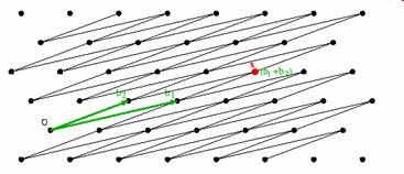
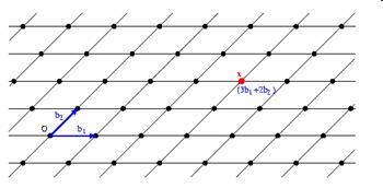
Thus begins the hunt for the "best" basis.
In order do find the
elusive "best" basis we must first define what such a set might look
like. We begin by noting that the since the switch between two basis of
any given lattice L corresponds to the multiplication by a unimodular
matrix (i.e. a matrix with determinant of 1) the determinant det(b1, b2,...,bn),
is the same for all possible basis of L. Thus we define this to be the
determinant of L. The Hadamard approximation for the (euclidean) length
of the elements bi states: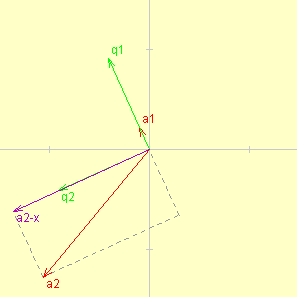
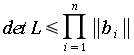
which holds true with equality if and only if the bi are orthogonal to each other. Thus the best we can hope for is an orthogonal basis. As a result we will now look at the process for orthogonalizing a given basis (in matrix form) which is called the Gram-Schmidt Orthogonalization. Intuitively this process can be understood as the transformation of a set of vectors into another set of vectors such that the new vectors are all pair wise orthogonal.
In the 2 dimensional
case shown in the graph to the right (taken from the excellent applet
by Nicholas Exner to be found at [U03]) the
original matrix (a1, a2)
consisted of the red vectors. First a1 is
normalized to form q1. Next the
projection of a2 onto q1
is subtracted from a2 to form the purple
vector which is then normalized to making q2.
Note that the normalization does not change anything about the space
being spanned and will therefor from now on, not be included in the
process anymore. Thus our final matrix will actually be (a1, a2-x).
This process can be generalized to the nth dimension as
follows. Given a set b1, b2,...,bn
of vectors over the real numbers (R^n), the vectors q1, q2,...,qn and the real numbers uij with i and j between 1 and n are
defined recursively as follows:
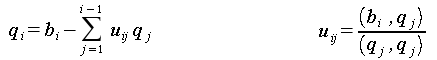
where "," denotes the ordinary inner product in R^n.
Since our stated aim is to form an equivalent basis for L
which is as orthogonal as possible (so as to get as close to the lower
bound given by Hadamard), we now lead to the following definition.
Definition 2.1: A basis (b1, b2,...,bn) is called size
reduced, if |uij|<
½ for all 1 < i < j < n.
In [LLL82] a simple algorithm for size reducing a
basis is given:
Algorithm 2.1: Size Reduction of a basis
Input:(b1, b2,...,bn)
for i = 2 to n do
//Size reduce column i of
the basis and of the matrix M=(uij)
for j =
i-1 downto 1 do
//Size reduce jth element uij
of column i
//round(x) rounds x to the nearest integer
//ui is the ith column of the
matrix M
bi = bi - round(uij) * bj
ui = ui -
round(uij) * uj
enddo
enddo
Note this algorithm does not change the Gram-Schmidt orthogonalized
basis.
At this point it is important to note that the
Gram-Schmidt process depends on the order of the vectors in the basis.
(This is why it was originally defined as an ordered set although this
is more then necessary when defining a lattice using the basis.) Now
from the definition of the Gram-Schmidt reduction we see that the
length of the size reduced basis gets smaller as the first vectors in
the Gram-Schmidt get smaller. Thus it is in our interest when trying to
find the most size reduced basis, to switch bi
and bi+1 in the original basis if this
results in the vector qi getting shorter.
Another reason to minimize the front vectors in the Gram-Schmidt
orthogonalized basis is the following theorem:
Theorem 2.1: If ||q1|| <
||qi|| for all i < n then q1 = b1 is the shortest vector in
the lattice
Thus this gives us a method for finding the shortest possible vector in
a lattice.
As a result we are now interested in finding a condition (in algebraic
terms) when we want to switch bi and bi+1. After some analysis which can be found in [LLL82] we conclude that we need to switch if the
square of the norm of bi is greater then
twice the square of the norm of bi+1.
Gathering results and putting everything formally we now have the
following definition:
Definition 2.2: A lattice basis (b1,
b2,...,bn) is called reduced
if
1. (b1,
b2,...,bn) is size reduced
2. ||qi||^2<
2*||qi+1||^2 for all 1 < i < n
which defines what our "best" basis actually looks like.
At this point it is worth noting that this is not the only definition
for a reduced basis. In fact a more intuitive definition (though sadly
less helpful as far as algorithm design is concerned) known as Minkowski
Reduced states that a basis B = (b1 ,
b2 ,…,bn) of a lattice L
is called Minkowski-reduced iff:
1. b1 is
the shortest nonzero vector in L
2. For i in [2,…,n], bi is the shortest vector in L such that (b1 ,…,bi) may be extended to a
basis for L.
Another more complicated but quite related, definition was given by
Korkin and Zolotarev, however it is a bit messy as it involves a rather
nasty formula and since we will not further need it I will leave it
out. One last note on the definition of reduced above, the
astute reader might notice that the second condition looks different to
the one in the original [LLL82] paper. However by
setting delta to 3/4 as it is in the paper a few lines of calculation
along with the Gram-Schmidt formulas show equivalence of the two
conditions. The alternate version was chosen for this paper as it is
more legible (involves half the variables) and is a slightly more
intuitive.
Now we have reached a point where we can begin thinking about algorithms to solve the problem. However first we need to define a constant B which gives us information about the size of the input vectors. This will be very useful in further complexity analysis as the runtime and communication overhead is often intrinsically tied to this value.
![]()
In [S86] and [GLS88] a
fundamental algorithm was given from which all approaches to compute
lattice basis reduction are derived. The algorithm goes as follows:
Algorithm 3.1: Basic Reduction Algorithm
Input: Lattice basis (b1 ,
b2 ,…,bn)
Output: Reduced lattice basis (b1 , b2 ,…,bn)
switch = TRUE
while (switch) do
Calculate the Gram-Schmidt
orthogonalized basis
as well as ||b1||^2
,…,||bn||^2 and the
matrix M
size reduce (b1 ,
b2 ,…,bn)
switch = FALSE
if (there exists an index i
with ||bi||^2 > 2 * ||bi+1||^2) then
switch =
TRUE
switch for
such an index i the vectors bi and bi+1
endif
enddo
Analysis of this algorithm has shown that at most n^2*log(B)
switches need to be performed before termination of a reduction, and the
calculation of the Gram-Schmidt basis requires O(n^3) operations
resulting in a total complexity of O(n^5*log(B)). There are two
main branches of algorithms which have been developed from the
algorithm 3.1. The first is often referred too as Stepping algorithms
which derive their name from the fact that they step through the basis
for k=2,...,n performing switches and then a
step back when ever necessary. The pseudocode for Stepping algorithms
is as follows:
Algorithm 3.2: Stepping Algorithm
Input: Lattice basis (b1 ,
b2 ,…,bn)
Output: Reduced lattice basis (b1 , b2 ,…,bn)
//Initialize k which holds the current step
k = 2
Calculate the Gram-Schmidt orthogonalized basis
as well as ||b1||^2 ,…,||bn||^2 and the matrix M
while (k < n) do
size reduce the kth column i.e. bk and uk using alg. 3.1
if (||bk||^2
> 2 * ||bk+1||^2) then
switch bk-1 and bk and fix qk-1 and qk in the
Gram-Schmidt orthogonalized basis
k = max{k-1, 2}
else
k = k+1
endif
enddo
Both the first polytime algorithm (LLL) as well as the improved version
presented by Schnorr and Euchner in [SE91] are
Stepping algorithms. From the pseudocode we can see that the interesting
parts to parallelize are the fixing of the Gram-Schmidt basis, the
calculation of the ||bi||^2's and
the size reduction of the kth columns of the basis matrix and
of M. Notice how this algorithm no longer requires the complete
recalculation of the Gram-Schmidt basis at every iteration but merely
its "repairing" in the form of an update to two columns. This fact
alone saves an O(n) operations per iteration resulting in a total
complexity of O(n^4*log(B)).
The second common approach derived from algorithm 3.1 is called the
Allswap algorithm and was first given in [RV92] by
Roch and Villard, however with out a proper analysis. This was later on
rectified by Heckler his dissertation [H95]. The
name comes from the property that instead of performing one switch of bi and bi+1 per
iteration the Allswap algorithms go through the entire basis and try
and switch as many bi's as possible
during each loop. In pseudocode:
Algorithm 3.3: Allswap Algorithm
Input: Lattice basis (b1 ,
b2 ,…,bn)
Output: Reduced lattice basis (b1 , b2 ,…,bn)
Calculate the Gram-Schmidt orthogonalized basis
as well as ||b1||^2 ,…,||bn||^2 and the matrix M
order = ODD
while (swapping still possible (i.e. there
exists an i such that point 2 of def. 2.2 doesn't hold))
size reduce(b1,
b2 ,…,bn)
if (order = ODD) then
switch bi and bi+1 for all odd
indices i where ||bk||^2 > 2
* ||bk+1||^2
order =
EVEN
else
switch bi and bi+1 for all
even indices i where ||bk||^2
> 2 * ||bk+1||^2
order = ODD
endif
Recalculate Gram-Schmidt basis and M
enddo
size reduce(b1 , b2 ,…,bn)
The analysis of this approach shows that now O(n^3) operations
are required per iteration since each time the entire Gram-Schmidt
reduction (and size reduction) need be recalculated! However since so
many swaps are being performed each loop, only log(B)*n
iterations are required before the shortest b1
is the shortest vector in the lattice. This is NOT the same as saying
the basis is reduced! However it is similar enough that for many
applications such as simultaneous diophantine approximation [S86], it suffices. As a result the complexity of the
two approaches 3.2 and 3.3 can for most practically purposes be
considered equal at this theoretical level (since log(B)*n loops
each with O(n^3) operations means a complexity of O(n^4*log(B)).
Another problem with 3.3 is that during the calculations significantly
larger numbers appear compared to 3.2. This can effect both the runtime
of the operations as well as the communication overhead when
parallelizing. The blow up can be quantified (theoretically) by noting
that the binary complexity of 3.3 is an order of n higher
then that of 3.2 (in the serial case)! Luckely practice has shown this
to be merely a theoretical worry though.
Now we turn to an implementation issue which has led
to some significant advancements in the runtime of lattice basis
reduction algorithms. One of the main reasons that the original versions
of both the Allswap algorithms as well as Stepping algorithms were slow
in practice was that all calculations were being done in arbitrary
precision (exact arithmetics). A much faster, though less
precise, alternative to this is floating point arithmetic. Though from
a mathematical point of view, this is quite undesirable as the
leveraging of this speedup causes some seemingly unnecessary
complications in the algorithm while introducing the problem of numeric
instability.
In [SE91] Schnorr and Euchner took the LLL Stepping
algorithm and modified it to use floating point arithmetic for all but
storing the lattice basis itself since any changes to that would
completely alter the lattice. To avoid problems with numeric
instability the following code was included:
Algorithm 3.1: Schnorr Euchner lattice basis reduction (only
relevant parts included in listing below)
Input: Lattice basis (b1 ,
b2 ,…,bn)
Output: Reduced lattice basis (b1 , b2 ,…,bn)
Note: t = number of precision bits of the floating point variables
the ' operator denotes
conversion from precise arithmetics to floating point
M is stored as a floating point matrix
...
//Calculate Gram-Schmidt coifs. uk and ||bk||^2
...
if( |transpose(b'k) * (b'j)| < 2^(-t/2) * ||b'k||
* ||b'j|| ) then
s = (transpose(bk) * (bj))'
else
s = transpose(b'k) * (b'j)
...
...
//Size reduce bk
..
if( |ukj|
> 1/2) then
u = round(ukj)
Fr = TRUE
if ( |u|
> 2^(t/2) ) then
Fc
= TRUE
endif
...
...
if (Fc) then
k = max{k - 1, 2}
else
//switch or increment k
endif
...
Thus both in the Gram-Schmidt update as well as in the size reduction
portion of the algorithm a step is included where the rounding error is
calculated. If the error in the Gram-Schmidt calculation is deemed to
large, then the calculation is first done in precise arithmetics and
only then converted to floating point. However if an error is
discovered during any step of the size reduction then k is simply
decremented with out a switch.
A rather different approach in dealing with rounding errors with the
floating point speed up was taken by Heckler and Thiele [HT98]
when they presented their Allswap algorithm based on the original
precise arithmetic algorithm by Roch and Villard [RV92].
They decided to recalculate the Gram-Schmidt basis and thus the entire
matrix M every iteration from the lattice basis which is always stored
in precise form. Thus errors can not compound and so don't pose a
significant problem anymore. (They proved this claim of course, with
careful analysis.) To avoid the O(n^3) cost of recalculating a
Gram-Schmidt basis each iteration they used a new algorithm which
hinges on a Givens rotation. This algorithm if properly parallelized,
can bring a speedup of O(n^2) on an n^2 processor grid
thus making that part of the algorithm linear!
The next step is to take all these different
approaches and begin the actual process of parallelizing them. There are
two parts in both approaches which can effectively be parallelized. The
size reduction (alg 3.1) and the Gram-Schmidt orthogonalization (or its
update). Also parallelization can be done either for n or for n^2
processors. The approach for the Gram-Schmidt parallelization for n^2
processors was mentioned above (use Givens rotation). To be more precise
though we refer to a paper by Schwiegelshohn and Thiele [ST87]
where it was shown that algorithms of the form:
Algorithm 3.2: Schwiegelshohn Thiele Parallelizable
Note: fij are all of a
special linear form
for i = 1 to n-1 do
for j = i+1 to n do
A = fij(A)
enddo
enddo
can be parallelized. such that the speedup on an n^2 processor
grid is of quadratic order. As Heckler pointed out in [H95]
both the Gram-Schmidt orthogonalization as well as the size reduction
can be expressed as algorithm 3.2 and can thus be sped up to linear
time on n^2 processors.
As for the case of parallelizing on n processors once again both
relevant parts of the algorithm are similar enough that we can on a
theoretical level, analyze them together. (When it comes to actual
implementation the differences will merely be expressed in the form of
symmetry. Where one is column distributed the other must be row
distributed. etc.) There are three ways to go about this problem. The
first and most obvious we will call the naive approach. In this method
all processors maintain a copy of the entire matrix M as well as the
basis (i.e the whole state of the problem) locally. Each computes a
predefined column and then distributes the result to all of its peers.
At this point we will make the distinction between the startup cost of
a communicating and the cost measured by data units (usually one
floating point value) sent. If the processors are arranged in a
hypercube then this method costs n times the startup cost and n^2
data transmissions. If however communication is done in serial such as
in a ring structure then this costs n^2 times the startup cost
as well as the data transmission costs. The operation count is
quadratic for the computation of a single column which is no speed up
over the serial case. (This is clear since for a single column this is
the serial case.) However for the entire matrix the remaining cost is
only in communication. No more operations need be performed, resulting
in a linear speed up over the serial case. Thus this is a viable method
for Allswap algorithms which recompute the en
The second method which was proposed in [H95] when
is known as the Pipelining method, and involves distributing
the matrix row wise for the size reduction. It can be understood as
calculating each size reductions (of the columns) sequentially but
parallelizing the process of calculating one such size reduction.
Therefore this method is applicable to both Allswap algorithms as well
as to Stepping algorithms. This process incurs a startup cost and data
transmission cost of n^2. But because values of M from the
previous round are used the problem of producing large numbers is
minimized in comparison to the other methods. The speedup is once again
optimal resulting in O(n) operations for the reduction of a
single column. The biggest drawback though is that, as one can see from
the first if-then statement in the listing of algorithm 3.1, if a
single processor fails this check, then the penalty of recalculating
the new value for s in precise arithmetic is incurred on all
processors as they must wait for the last processor to finish its
calculation before the next column can be processed!
The last method which was first presented in [RV92]
can be thought of as the dual to the Pipelining method. It is called the Cyclic
method and calls for the Gram-Schmidt matrix M as well as the lattice
basis matrix to be distributed row wise over the processors. The
calculations of the size reduction of each column is then done in
parallel with the steps being done in serial. This method only calls
for n/2 processors as each one maintains two rows of the
matrices. The startup cost is reduced to n but the data
transmission cost is still n^2.One problem with this algorithm
is that it has the greatest potential to form large numbers which is
detrimental to the numerical stability, runtime, and communication cost
of the entire lattice basis reduction. Since all columns are calculated
in parallel this is not a viable method for Stepping algorithms,
however for Allswap algorithms were the entire matrix needs to be
recalculated in one go, this method makes a linear (optimal) speed up
on n processors possible.
Now that we have covered the rather broad spectrum of possibilities at hand, it becomes clear that we need to reasons for choosing amongst them, as there is no single approach that is better then the rest for all cases. The first and probably most important criterion when designing the approach is to specify the type of supercomputer being used. Specifically the choice between a SIMD or MIMD computer must be made. In our case, that of MIMD, this means we have a rather limited number of processors at hand and will thus opt of schemes optimized for n CPUs. Another point speaking for MIMD machines is that all approaches call for, at one point or another, each processor to perform different (asynchronous) operations at the same moment in time. On a SIMD machine this requires sperate time units for each different operation since during any given time unit either a process is performing a single specific task or waiting which would not allow us to leverage the full theoretical speedup of our parallelized. algorithms. (The case of implementing a parallel algorithm on a computer grid, or distributed network using a library such as LiPS for example can be considered analogous to a MIMD super computer at this point. The only difference for parallel lattice basis reduction being that communication costs are proportionally even higher.)
When deciding between the Stepping algorithm approach and the Allswap approach it is very helpful to highlight their differences. The table below compares the best options for parallelizing on n processors. Note: values are the order in O notation i.e. not precise.
|
|
Algorithm |
1. Allswap with Cyclic Gram-Schmidt and size reduction |
2. Allswap with Cyclic size reduction and local computation Gram-Schmidt(*)(***) |
3. Stepping with Pipelining Gram-Schmidt and size reduction |
4. Stepping with Pipelining Gram-Schmidt and Naive size reduction (*) |
|
|
Phases |
n |
n |
n^2 |
n^2 |
|
Size Reduction |
Operations per phase |
n^2 |
n^2 |
n |
n |
|
Startup cost per phase |
n |
n |
n |
n |
|
|
Data transmission cost per phase |
n^2 |
n^2 |
n |
n |
|
|
Gram Schmidt |
Operations per phase |
n^2 |
n^3 |
n |
n^2 |
|
Startup cost per phase |
n |
0 |
n |
0(**) |
|
|
Data transmission cost per phase |
n^2 |
0 |
n |
0 |
(*) requires both matrices to be stored locally at each processor
(**) assuming a hypercube topology
(***) local computation means each processor
computes the complete Gram-Schmidt orthogonalization from its local
data.
First of all we can split these four options into two categories. There is a trade off between having n^2 (or n^3 if one doesn't want to risk large numbers and thus uses a stepping algorithm instead) startup costs and n^3 data transmission during the Gram-Schmidt reductions (options 1 and 3) and having no communication at all during the Gram-Schmidt phase but therefore having a quadratic operations cost (options 2 and 4). Also 2 and 4 require an order of n more memory for each process. However since we are working on a MIMD machine with a relatively slow network (Fast Ethernet) compared to the computational power of any given CPU, and because each CPU has approximately 256MB of memory available and n can will be relatively small in practice (<256) we will opt for either 2 or 4. (A quick calculation shows that even if n = 256 then 256 * 256 * 2 matrices * 600 bit / (8 bits per byte * 2 ^ (20) bytes per MB) * 16 processes per processor = 150 MB. Already n = 256 would take several hours to terminate on a 16 CPU machine.) Finally, by deciding for the Allswap algorithm (option 2) we can avoid the problem of having to calculate the Gram-Schmidt part with precise arithmetics (see alg.3.2) by using Givens Rotation as suggested be Heckler and Thiele and at the same time avoid unnecessary network startup costs during the size reduction section while keeping the same complexity level of total operations as in option 4.
When it comes to the language to be used for
implementation there are two main choices which present themselves. C
based using MPI as a communication library, or Matlab*p. At this point
it is not really clear for a performance point of view whether one or
the other would be preferable. However, so as to facilitate porting
this code to other clusters which will most probably not have Matlab*p
installed (such as the one I am working on at my university in Vienna)
I have opted for C and MPI (as I happen to know this is supported on
the machine I will hopefully be continuing this project on).
We have seen that parallelizing lattice basis
reduction is intrinsically tied to the theoretical structure behind the
problem. (Orthogonal basis imply the lower bound in the Hadamard
approximation so we look at the Gram-Schmidt orthogonalization. process
whose coefficients become a measure of how reduced our basis is, for
example.) There are two distinct branches, Stepping algorithms and
Allswap algorithms, each with its advantages and disadvantages. Both
however greatly benefit from leveraging the speed of floating point
calculation, which shows that to truly attain optimality it is
important to consider implementation issues as well as theoretical
ones. Next we looked at how the two basic computationally intensive
parts (size reduction, and Gram Schmidt orthogonalization) can be
parallelized. We noted how each has its own strong and weak points
(Memory vs Communication cost, etc.) and how some can only be applied
to certain algorithms (Cyclic only works for Allswap, etc.) thus the
choices that need to be made when implementing a parallel lattice basis
reduction algorithm depend heavily on the environment at hand. What
type of computer (MIMD, SIMD, distributed workstations), what order of
processors compared to the values of n being computed, what are
the costs of communication (startup, data transfer), what topology
(grid, ring, serial,...), how much memory does each processor have
compared to the data it must handle and what are the requirements on
portability of the code. Each one of these questions has its own
implications and can effect the final product and must therefor be
taken into consideration. As such given the "tools" presented here it
is impossible to create an all purpose "best" algorithm, but on the
other hand for each environment there is a given combination of tools
which will produce the best results.
[B89] J. Boyar. Inferring sequences produced by pseudo-random number generators. J. of the ACM, 36(1):129-141, January 1989.
[BM01] J. Blomer and A. May. Low secret exponent RSA revisited. In Cryptography and Lattices - Proceedings of CALC '01, volume 2146 of LNCS, pages 4-19. Springer-Verlag, 2001.
[C91] B. A. LaMacchia M.J. Coster, A. M. Odlyzko, and C. P. Schnorr. An improved low-density subset sum algorithm. In EUROCRYPT '91, 1991.
[C97] Don Coppersmith. Small solutions to polynomial equations, and low exponent RSA vulnerabilities. Journal of Cryptology, 10(4):233--260, 1997.
[DN00] G. Durfee, P. Nguyen, Cryptanalysis of the RSA Schemes with Short Secret Exponent from Asiacrypt '99", Proc. of Asiacrypt '2000
[FHK88] A. M. Frieze, J. Hastad, R. Kannan, J. C. Lagarias, and A. Shamir. Reconstructing truncated integer variables satisfying linear congruences. SIAM J. Comput., 17(2), April 1988.
[GLS88] M. Grötschel, L. Lovasz, and A Schrijver. Geometric Algorithms and Combinatorial Optimization. Springer-Verlag, 1988.
[H95] Christian Heckler. Automatische Parallelisierung und parallele Gitterbasisreduktion. Dissertation, Institut für Mikroelektronik, Universität des Saarlandes, Saarbrücken, 1995.
[HT98] C. Heckler and L. Thiele, Complexity analysis of a parallel lattice basis reduction algorithm, SIAM J. Comput. 27 (1998), no. 5, 1295--1302 (electronic).
[LLL82] A. K. Lenstra, H. W. Lenstra, and L. Lovász. Factoring polynomials with rational coefficients. In Math. Annalen 261 pages 515-534, 1982.
[LO83] J. C. Lagarias and A. M. Odlyzko. Solving low-density subset sum problems. In Proc. 24th IEEE Symp. on the Found. of Comp. Sci., pages 1-10, 1983.
[NS01] P. Q. Nguyen and J. Stern. The two faces of lattices in cryptology. In Proc. Workshop on Cryptography and Lattices (CALC '01), volume 2146 of LNCS. Springer-Verlag, 2001.
[RV92] J.L. Roch and G. Villard. Parallel gcd and lattice basis reduction. In Proc CONPAR92 (Lyon), LNCS 632, pages 557-564. Springer Verlag, 1992.
[S82] A. Shamir, A polynomial-time algorithm for breaking the Merkle-Hellman cryptosystem, In Proc. 23rd IEEE Symp. on the Found. of Comp. Sci., pages 142-152, 1982.
[S86] A. Schrijver. Theory of Linear and Integer Programming. John Wiley and Sons, 1986.
[SE91] C.P. Schnorr and M. Euchner. Lattice basis reduction: Improved practical algorithms and solving subset sum problems. In Proceedings of the FCT'91 (Gosen, Germany), LNCS 529, pages 436-447. Springer, 1984
[SH95] Schnorr and Horner. Attacking the Chor-Rivest cryptosystem by improved lattice reduction. In EUROCRYPT '95, 1995.
[ST87] U. Schwiegelshohn and L. Thiel. A systolic array of cyclic-by-rows Jacobi algorithms. Journal of Parallel and Distributed Computing, 4:334-340, 1987.
[U03] N. Exner, http://www.mste.uiuc.edu/exner/ncsa/orthogonal at the University of Illinois At Urbana-Champaign.