
MIT 18.337J Parallel and Scientific Computing
Parallelizing a 2D Kolmogorov-Smirnov Statistic
Ian Chan
PowerPoint Slides: http://web.mit.edu/ianchan/KS2D/ks2dpres.ppt
Abstract:
Kolmogorov-Smirnov(KS) Test is a very popular non-parametric statistic for comparing 2 empirical distributions in the 1 dimensional case. Several 2D dimensional analogue exist and they are widely utilized in analyzing large datatsets such as astronomical data from microwave telescope to geological recordings to financial data analysis. This project attempts to parallelize one version of the 2D KS test proposed by Peacock[1,2]. A serial O(nlogn) algorithm (muac) has been devised by Cooke[3] that utilizes binary tree data structures. Achieving optimal load balancing by random sampling of input data and online adaptation to inputs are employed. The results show that as more sample size becomes large, we see the advantages of the parallel algorithm. The parallel algorithm also enables the processing of larger samples and thus, reap gains in speed as well as problem size.
Table of Contents
3.2 Serial O(n log n) algorithm with Binary Tree Data Structure (Muac)
3.2.1 Pseudocode
3.3.1 Pre-sorting
3.3.2 Load balancing
3.3.3 Finding max(D) by Downward Tree Traversal(Serial Algorithm)
6. Conclusion
7. References
1. Proposal and Motivation
Kolmogorov-Smirnov(KS) Test is a very popular non-parametric statistic for comparing 2 empirical distributions in the 1 dimensional case. Several 2D dimensional analogue exist and they are widely utilized in analyzing large datatsets such as astronomical data from microwave telescope to financial data analysis. Because the need to compare two empircal distributions arise often in research and engineering applications involving large volumes of data, it would be useful to implement a parallel version that can ease computational time and data storage requirements. There is no existing 2D KS test in the statistical toolbox currently and would be a nice feature for MATLAB or MATLAB*P.
Although no bounds have been proven for this version or other verions of the 2D KS test (unlike the 1D case proven by Brownian bridge arguments), the bounds have been verified by large Monte Carlo simulations and is therefore a reasonable statistic.
This project attempts to parallelize one version of the 2D KS test proposed by Peacock[1]. A serial O(nlogn) algorithm has been devised by Cooke[2] that utilizes binary tree data structures. Details of the KS test and the algorithm can be found in subsequent sections.
2 KS Test Introduction
2.1 1D KS Test
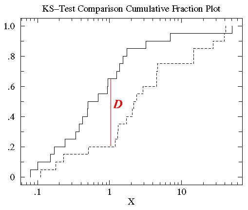
The standard 1D KS test compares two empirical sets of data and determine they come from the same distribution. The D statistic is the largest difference between the two empirical cumulative distribution function (cdf) Fm and Gn. Fm denotes empirical distribution Fn has n samples and empirical distribution G has m samples. The bound for the 1D test is:
Diagramatically, the D statistic is illustrated in the following figure:
One can parallelize this procedure by sending chunks of data to different processors and combining the cdf from
each processor at the end for find the maximum difference, the D statistic. This is an embarassingly parallel procedure.
2.2 2D KS Test
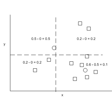
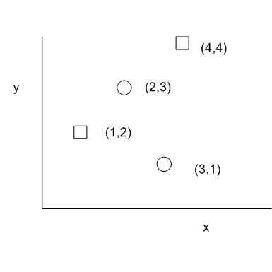
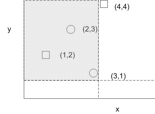
This version of the 2D analogue of the KS Test by Peacock has been used to analyzed astronomical data. It is attractive because it has a bound similar to the 1D KS test and has been validated by Monte Carlo simulation. The test statistic is based on the quadrant in which the difference in the number of observed points from the 2 groups is largest. In other words, all possible center point of the quadrants are explored such that we find that quadrant that maximizes abs(fraction of data from group F - fraction of data from group G). This quantity is the D statistic for this 2D KS test. The following figure illustrates the D statistic. Squares and circles represent samples from two different data sources. The quadrant with a large D statistic contains a large population from one group while a small population from the other group.
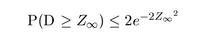
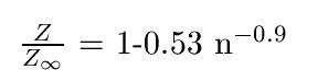
Let s = nm/m+n where m and n are the number of samples in each empirical distribution, the empirical bound of the D statistic for the 2D KS test can be found as follow where Z(n) = sqrt(n) * D
3 Algorithms for 2D KS Test
3.1 Brute Force Algorithms
If we loop through the center of the quadrant axes, our algorithm would be O(n^2). However, this algorithm does not consider all possible quadrants. The example given in the previous section is an example. The center of quadrant axes in the example does not lie on (or near) one sample, it has x-coordinate of one sample and a y-coordinate of another. To loop through all possible centers of quadrant axes require an algorithm of O(n^3).
3.2 Serial O(n log n) algorithm with Binary Tree Data Structure (Muac)
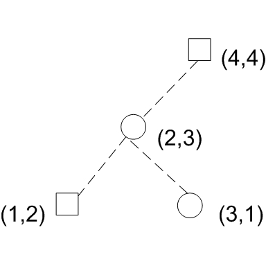
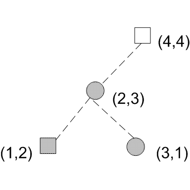
The following algorithm proposed by Cooke[3] runs in O(nlogn) time and O(n) space. It considers the top 2 quadrants and bottom 2 quadrants separately. For the top 2 quadrants, the algorithm sweeps down from top to bottom on the y axis, constructing a binary tree and adding a node for each data sample encountered on the sweep. Assuming that data is sorted by y, the following diagram illustrates the tree construction process. Notice that in the binary tree, the left child's x is always smaller than the parent's x and the right child's x is always greater than the parent's x.
This data structure presents several interesting features related to the actual 2-D data distribution:
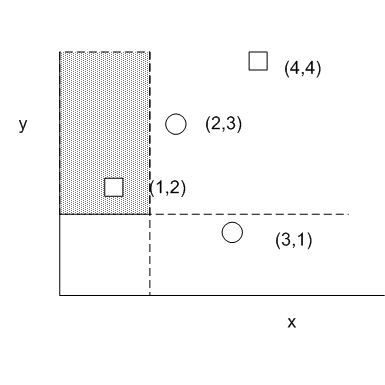
Consider how this data structure can be useful in the computation of the 2D KS statistic, the maximum difference between the density of two groups among all possible quadrants. We need to be able to find the density of all possible quadrants. Suppose we consider the top left quadrant only. One can draw quadrants such that it only includes the leftmost point, which corresponds to the following tree representation..
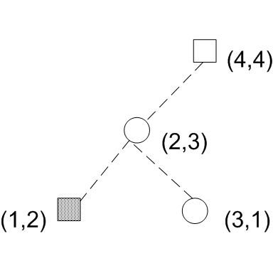
Suppose we define D = Fs - Fc where Fs is the cumulative density of s in a particular quadrant. This situation represents a D statistic of (1/Ns - 0/Nc) where Ns is the total number of square samples and Nc is the total number of circle samples. Likewise, if we set the quadrant such that it includes (3,1), the quadrant must include 3 points:
Notice that if we include a right child in the quadrant, we must also include its parents and all it's left children. In this case, we have at node (3,1) a D statistic of (0/Ns-1/Nc) + delta, where delta is the cumulative difference at node(2,3) which is 0 since node(2,3) and all its children( node(1,2) only in this case) have 0 difference in cdf (1 square and 1 circle -> 0 difference in cdf's).
The algorithm works as follows. Finding D is also finding quadrant Q, which is the quadrant that has the maximum D statistic. After building this binary tree data structure, we start at each of the childrenless nodes and propagate up. For example, suppose we start at the childrenless nodes (1,2), D would be 1/Ns. We then propagate upward to its parent (2,3). The parent now decides among 3 choices for D:
In this sample case, (2,3) had both left and right child. If one of the children is missing, the choices for D would be limited to 2. Since we are trying to find the maximum D, the parent chooses by taking the maximum of the 3 choices.
Because we are looking for abs(difference), both the minimum and the maximum is kept at each node. delta of each node is the total difference in density iff the node and all its children are included in the quadrant. As shown in the pseudocode in the following section, the serial algorithm propagates up the tree after adding each node(data point) to the tree. This is not the most efficient way to calculate the maximum/minimum.
3.2.1 Pseudocode
main:
for (x,y) = data pairs
 node = newnode(x,y)
 tree.addnode(node)
 tree.propagateup(node)
 maxDelta = MAX( MAX( root->max ), -1 * MIN( root->min))
end


tree.propagateup(node):
for (node; node != null; node = node.parent) if ( node->left && node->right) node->delta = node->left->delta + node->score + node->right->delta node->min = MIN( MIN( node->left->min, node->left->delta + node->score ), node->left->delta + node->score + node->right->min ) node->max = MAX( MAX( node->left->max, node->left->delta+ node->score), node->left->delta + node->score + node->right->max ) else if (node->left) node->delta = node->left->delta + node->score node->min = MIN( node->left->min, node->left->delta + node->score) node->max = MAX( node->left->max, node->left->delta + node->score) else node->delta = node->score + node->right->delta node->min = MIN( MIN( 0, node->score ),node->score + node->right->min) node->max = MAX( MAX( 0, node->score ),node->score + node->right->max) end
3.2.2 Searches on other 3 quadrants
We have described the search for the top left quadrant. Searches on the other 3 quadrants are analogous. For example, D statistic for the top left and top right quadrants can be calculated using the same tree structure. Instead of choosing between left_min, left_delta+score and left_delta + score + right_min, we will be choosing between right_min, right_delta+score+left_min. The bottom 2 quadrants can be found using the same algorithm by simplying chaning sorting the inputs by decreasing y instead of increasing y. One can see the nice symmetry in this problem. The overall algorithm runs in O(nlogn) because the pre-sorting takes O(nlogn) and each of the 4 quadrant search requires looping through all input data O(n) and propagating up to the root O(log n ), yielding a total performance of O(nlogn).
3.3 Parallel Algorithm
Because the sequential addition of tree nodes is necessary for the algorithm to work correctly, the tree building portion of the algorithm cannot be parallelized. However, we can parallelize the upward propagation of the tree to find the minimum/maximum at the root node. There are two issues to watch:
3.3.1 Pre-sorting
Assuming that a parallel version of the quicksort algorithm is in place, we can sort the data by decreasing y values just like the serial algorithm. The gains of parallel quicksort relies on the ability to divide the list evenly among the processors in the early divide steps. This problem of load-balancing is similar to the one we face in implementing this algorithm.
3.3.2 Load Balancing
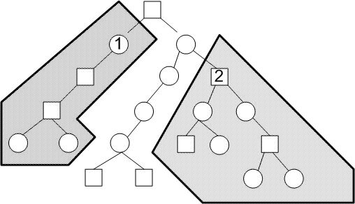
We would like to divide the binary tree near the root into n pieces, where n is the number of parallel processes. Suppose we have 3 processes, ideally the algorithm can divide the work evenly among the processors. If there are 3 processors(0,1,2), an equal division of labor is represented by the following figure. Each processor should acquire an equal number of nodes.
Suppose all the points in the group 1 above are in the interval [-inf, X1] and the points in group 2 are in the interval of [X2, inf]. To pick the appropriate sample interval breakpoints X1 and X2, we randomly sample min(s, 1000) points from the data and sort it by the x values. s is the total number of samples from the combined empirical distributions. We then find the (1000/n)th, 2(1000/n)th, ...(n-1)(1000/n)th x values and use them as the interval breakpoints for each of the processors. It is hoped that these x thresholds will evenly divide the the tree into more or less equal subtrees.
The drawback of the previous approach is that it is assumed that the samples are drawn from a distribution that have more or less independent x and y. Because the data is sorted by y, it may be true that for smaller values of y, x is small but for larger values of y, x is big. Therefore, we adaptively adjust the interval breakpoints adaptively. As we add new data to each processor, we keep a running average as well as sample counts in each processor. At every 1000 samples, we enter a checkpoint to see if the sample counts are too different (bad load balancing). In that case, we take the midpoints of the running averages as new interval breakpoints and continue the tree construction.
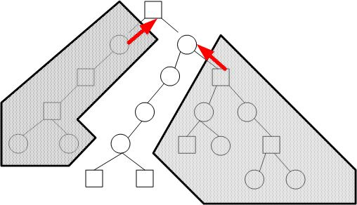
The red arrows indicate the inter-processor communications that have to take place. . We want to improve speed by intelligent partitioning of the tree so that we minimize inter-processor communications.
3.3.3 Finding Max(D) by Downard Tree Traversal (Serial Algorithm)
Unlike the serial algorithm that propagates up the tree each time a node is added, the parallel algorithm constructs the entire tree first without recalculating intermediate nodes of the trees. Upon completion of the tree construction, we start at the node and traverses down the tree recursively to find the maximum D. The recursive algorithm pseudocode is given below:
recur-max-min-delta(node)
[maxleft, minleft, deltaleft] = recur-max-min-delta(node.leftchild)
[maxright, minright, deltaright] = recur-max-min-delta(node.rightchild)
max = MAX(maxleft,
          deltaleft+node->score,
          deltaleft+node.score+maxright,
          node->score)
min = MIN(minleft,
          deltaleft+node->score,
          deltaleft+node.score+minright,
          node->score)
delta = deltaleft+node->score+deltaright

return [max,min,delta]
As with the serial case, we will compare the max and -1*min at the root node to determine the max(abs(D)) for the entire tree. An important issue to consider here is that there will be waiting time if the tree constructions in each processors take different amounts of time to complete. Also, there will be a second waiting time if a process A in charge of a subtree needed by another process B does not finish calculating the [max,min,delta] for A. Therefore, it is important for the subtree branching points to occur near the top of the entire tree.
3.3.4 Upward Tree Traversal (Parallel Algorithm)
After populating the trees in each processor, we work upward from the bottom of the trees by considering each node in a LIFO (last in first out) fashion. We look at the node that is last added to the tree first and that node should be a childless node. As we propagate upward in each processor, we might run into a node that waits for the results from its child, which is hosted by another processor. This processor is locked until the other processor gets to that node. There will be no locking because there is not circular path in a tree. But good load balancing is necessary to prevent excessive dead time.
You can find the source code for the MPI implementation here.
We have looked at sample sizes = 10,000 and 100,000 (N1 and N2) with 1, 2, 4, and 8 processors. The results are shown below.
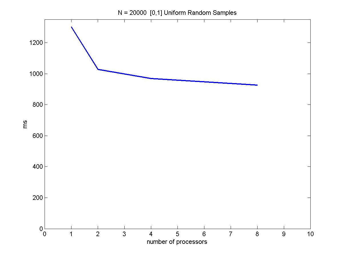
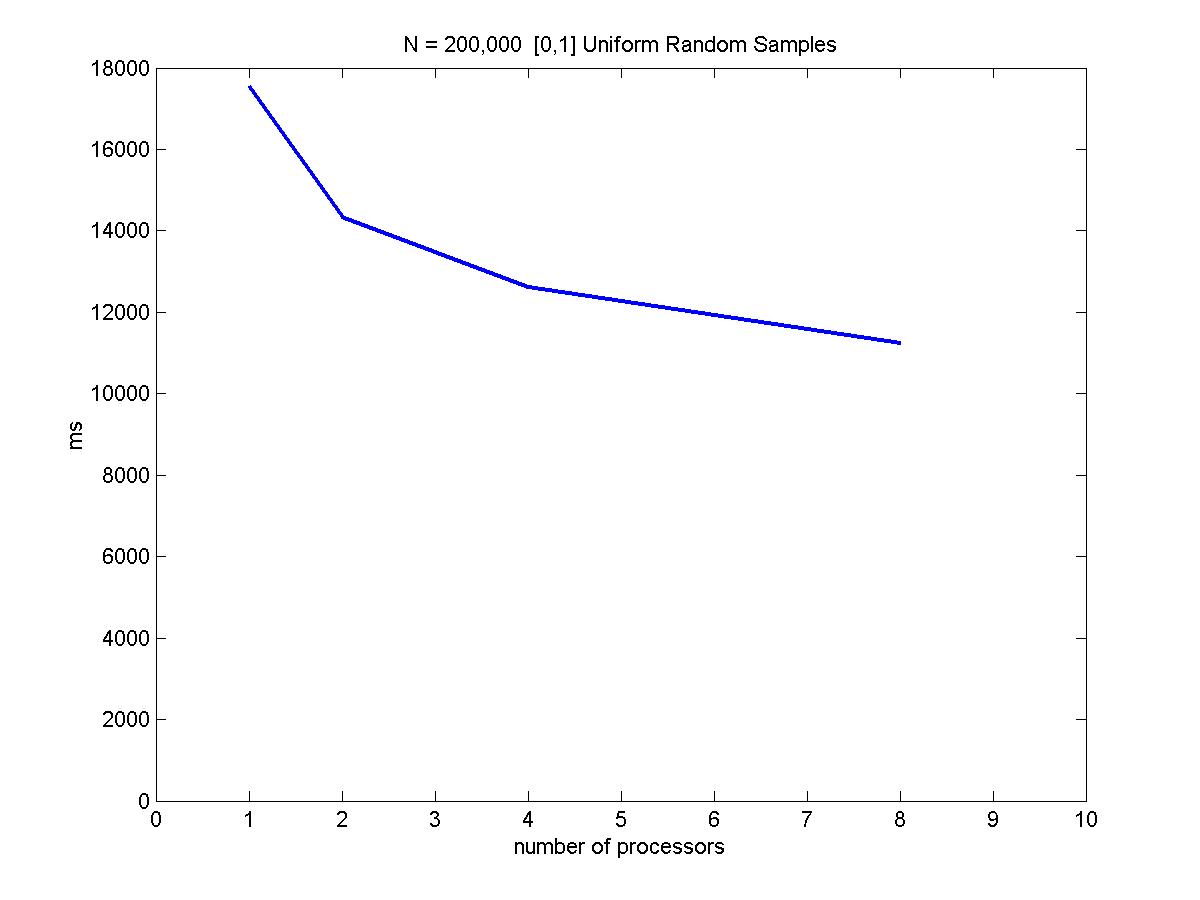
Because these samples are randomly drawn from a uniform [0,1] distributions, x and y are independent and the random sampling load balance scheme discussed in earlier sections apply well in this situation. Notice the speed up is not linear because the tree building portion of the algorithm is not parallelizable. Also, increasing # processors would also add more inter-processor communication overhead to the performance.
Considering another data distribution, we plot the performance vs # processors for 100,000 again. The samples are drawn form standard normal distributions centered at (-0.7, 0.7) and (0.7, -0.7). The standard deviation is 1. We use a checkpoint of every 1000 points to adaptively re-partition the interval breakpoints. (this techique was discussed in an earlier section). The results are shown below.
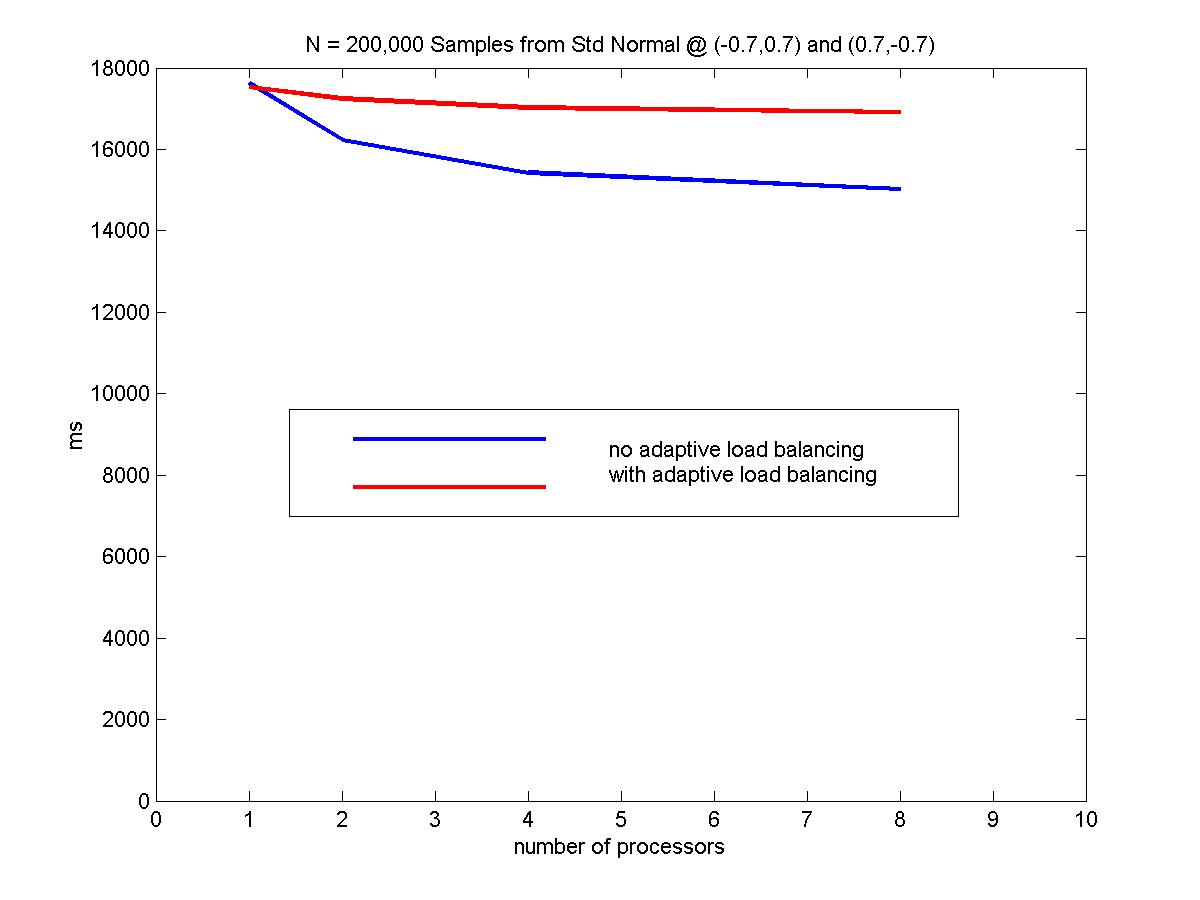
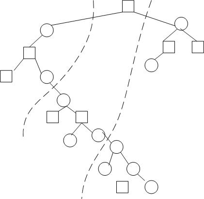
Notice that without adpative load balancing, the parallel algorithm has almost the same performance as the serial version. This is the case because the tree is divided such that for large values of y, most of the work is assigned to processor 0 but for smaller values of y, it is assigned to processor N. Processor 0 needs to wait for the results of processor N to proceed in this current implementation. The "relay" situation is not doing any better than a single processor doing all the work. As an example, the following figure illustrate a distorted tree that can cause problems in the current implementation. A better implementation would be to do use a "garbage collector" approach and up-propagate any nodes that can be up-propagated without waiting for the results from other processors. However, the implementation would be more tricky and requires backtracking to see if the skipped over node is ready.
Although we did not observe linear speedups after parallelization, this parallel version of the 2D KS test is still practical because it allows the solving of a samples size larger by a constant multiplier factor. There is no single heuristic of load-balancing the tree data structure in this problem because the shape of the tree largely depends on the distribution of the data. Several methods of load balancing has been explored here in this project and has been demonstrated to boost performance from the gathered performance data.
[1] Peacock J, Monthly Notices of the Royal Astronomical Society, 1983, vol 202 p615: Two-Dimensional Goodness-of-Fit Testing in Astronomy
[2] Fasano G, Franceschini A. Monthly Notices of the Royal Astronomical Society, 1987 vol 225 p 155: A Multidimensional Version of the Kolmogorov-Smirnov Test
[3] Cooke A. The muac algorithm for solving 2D KS test by http://www.acooke.org/jara/muac/algorithm.html
[4] Cormen, Leiserson, Rivest. Introduction to Algorithms MIT Press 1990