Rendering
We used Mesa3D graphics library, a "software" version of OpenGL,
to render the data. Since standard OpenGL renders directly to the
graphics card memory, we needed Mesa3D library which renders
graphics to arbitrarily chosen location in processor's main (RAM)
memory.
Rendering Pipeline
- A processor is given the width and the height of the entire
image.
- It communicates to the main node whether or not it has any
data on its node; thus, when the main node decides to gather the
pixel buffers once the data has been rendered it knows which
processor to expect the data from and which one to ignore.
Processors also communicate the maximum and the minimum value in
their data buffers which is needed for correct display of surf and
mesh functions.
- Each processor renders the portions of matrix data located on their
respective nodes to their memory buffers. They use a 64-color
color map from matlab as a color table. Thus each pixel is
represented as an 8-bit unsigned char which considerably reduces
transfer time of pixel buffers.
- Once the data has been rendered a processor can either send the
entire pixel buffer or compute the bounding box around the
"damaged" pixel buffer data and send only that box (one can choose
one option or the other by including #define _RECTANGLE_ in
render.cc). The advantage of using a rectangle is that less data
is sent to the main node. At the same time the main node has to
use blocking receives because it needs to know the size of the
bounding box before it receives the pixel data. If one does not
use the bounding box method, main node always (non-blocking) receives
the entire image buffer from all the nodes.
In the case of 3D plots (surf and mesh) each processors sends
along pixel color values a pixel depth buffer, so that the main
node can do proper z-buffering and image overlaying.
- After it received the pixel buffers, main node writes them over
its rendered data. In the case of spy, it writes every non-white
pixel received. In the case of the 3D plots it writes only those
pixels that are closer to the viewer than the ones it (the main
node) rendered.
- Main node converts pixels from 8-bit indices in the
color map to RGB data and returns the RGB data to the calling
function.
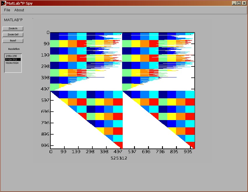
Ppspy
Ppspy's output differs slightly from regular Matlab
spy. Namely, we decided to color data from each individual node
differently so that in addition to getting information about the
matrix data you also get the information about its layout on
the cluster.
The following figure shows the output of a 1024x1024 matrix
distributed on eight nodes (hence eight different colors):
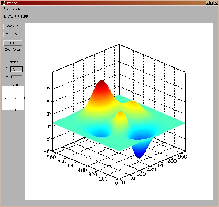
Ppsurf
Ppurf command let's user view the surface created by the matrix
data where x, and y coordinates correspond to matrix row and
column indices and z coordinates are the actual value of matrix
data. We support zooming feature as well as rotation around z and
x axis.
The surface plotted using ppsurf looks identical to the one
plotted using surf command. The only difference is that we create
gaps in surface between the data blocks that were laid out on different
nodes. While we could have filled these gaps by exchanging
bordering row and column data between the nodes, we didn't do it
for performance reasons. In addition, since ppsurf command is
invoked only on matrices larger than 1024x1024 (and the block size
on individual node is never greater than 64x64) these gaps are
practically invisible to the user.
The following figure shows the output of a "peaks" matrix(1024 x
1024):
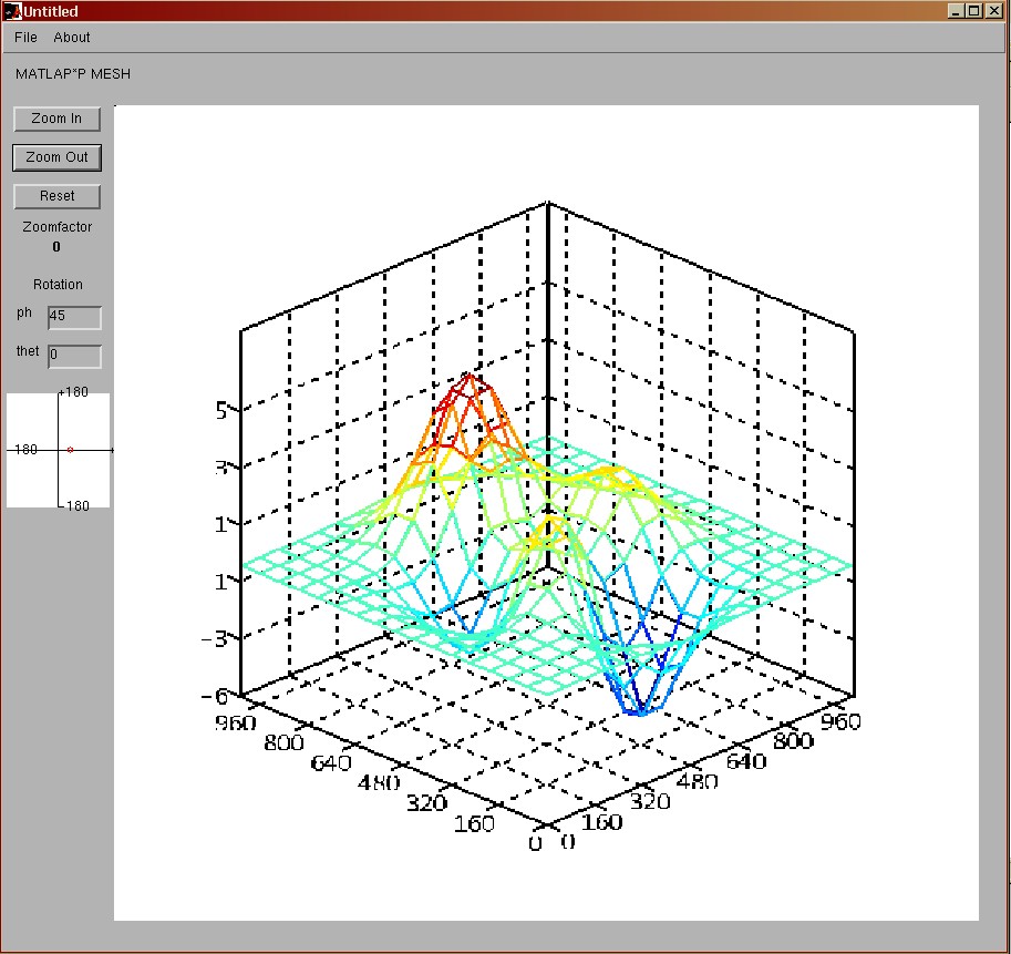
Ppmesh
Ppmesh is very similar to ppsurf with the only difference that we
only render the corner nodes of each 64x64 data block. Thus, even
for large matrices the resolution is usually big enough to view
the surface as a mesh rather than a solid (which is what mesh
command does).
The following figure shows the output of a "peaks" matrix(1024 x
1024):
Rendering Files
- render.h render.cc - rendering "kernel" that draws and communicates
the pixel data between the nodes.
- spyrender.h spyrender.cc - rendering specific to spy command
- tdrender.h tdrender.cc - rendering specific to 3D
commands (surf and mesh)
- surfrender.h surfrender.cc - rendering specific to surf
command
- meshrender.h meshrender.cc - rendering specific to mesh command