The following is my 6.338J/18.337J final project, as well as my Course 6 Advanced Undergraduate Project. I have written a parallel radiosity solver that runs in real-time on a cluster.
In addition to this web page, you can read my PowerPoint presentation. A project report document will be upcoming in the future. For now, this web page is the report.
A Brief Introduction to Radiosity
In 3D graphics, there are -- broadly speaking -- two steps that must be performed to decide the color of any pixel on the screen. The first step, often called hidden surface elimination, is to determine which object in the scene is closest to the eye along that line of sight. In real-time 3D graphics, this problem has essentially been solved by the Z-buffer algorithm. The second step, which is much more complicated, is shading -- the determination of how much light the eye is receiving from that object.
The simplest shading algorithms, and those used in the vast majority of real-time 3D applications, are local lighting algorithms. These algorithms add up the contribution from each light source in the scene to that particular location on the object. The essential property of all local lighting algorithms is that they do not take into account interreflections between objects -- they typically only handle a single reflection of a ray of light, from light source to object to eye. The great advantage of local lighting, however, is that it is easy to write out precise closed-form expressions for the intensity of the surface, which can be evaluated easily either at every pixel on the screen, or (in Gouraud shading) at each vertex of every object, and then interpolated.
An example of such an equation for local lighting is:
d-2(Md(N · L) + Ms(N · H)s)
N, L, and H are unit vectors. N is perpendicular to the surface. L points towards the light source. H is the unit vector pointing in the direction L + E, where E is the unit vector pointing towards the viewer. Md is the diffuse reflectance of the material, Ms is its specular reflectance, and s is a shininess coefficient, higher if the material is smoother. d is the distance from the surface to the light source.
In addition, a light color may be multiplied in. An emissive term may be added if the surface is glowing, and an ambient term may be added to make the scene brighter, as if there were interreflections.
It is now generally feasible on commodity graphics hardware to apply an equation of this complexity to every pixel of every object in a scene of moderate complexity. Shadows have proved more difficult, but stencil buffer shadow algorithms are generally robust and efficient enough to be used in real-time applications; such algorithms accurately compute shadowing for every pixel on the screen. These are "sharp" shadows, as opposed to soft shadows. Soft shadows can be approximated by using many light sources to approximate an area light source, though the performance burden of this can grow to be excessive.
Local lighting has proved a remarkably sound approach to shading, to the extent that even the complex RenderMan shaders used in CGI movies are typically still locally lit. However, in many scenes, especially indoor scenes, local lighting proves inadequate.
Radiosity (and its close relative, global illumination) takes a very different approach, by handling all interreflections.
Global illumination refers to algorithms that handle generic lighting models; radiosity specifically only attempts to solve the problem of diffuse lighting. Diffuse illumination is simple because surfaces appear to have the same brightness from any view direction; and most (though not all) interreflection in scenes tends to be of the diffuse variety.
Unfortunately, these algorithms pay a price for their accuracy in performance and memory consumption. Historically, they have been unsuitable for real-time rendering.
It is fairly easy to write out the basic equations for radiosity.
Suppose that there are n surfaces in the scene. Let Ai be the area of surface i. Let Ei be the amount of light energy emitted from surface i per unit time and area. Let Bi be the amount of light energy emitted and reflected from surface i per unit time and area. Let pi be the diffuse albedo of surface i in the frequency of light in question. Let Fij (called a “form factor”) be the fraction of light from surface i that reaches surface j.
Then, for all i, we must have:
AiBi = AiEi + pi sum(j in [1,n]: AjBjFji)
This is simply a linear system with n equations and n unknowns. It can be simplified further, given the identity that AjFji = AiFij, which can be derived from the quadruple integral that defines the Fij's:
AiBi = AiEi +
pi sum(j in [1,n]: AiBjFij)
Bi = Ei +
pi sum(j in [1,n]: BjFij)
B = E + RB
where Rij is piFij. The F matrix can be computed using the standard "hemicube" algorithm, which can be hardware-accelerated quite easily. (I will not present the detailed algorithm for the computation of F, or its precise definition.)
We can solve this either directly or via iteration.
The direct solution is easy to derive:
B = E + RB
B - RB = E
(I - R)B = E
B = (I - R)-1E
...but, unfortunately, it takes too long to compute. The iterative solution is much faster. If E is a local lighting solution, call it B0. Now let Bi+1 = B0 + RBi. Then, Bi is very simply the lighting solution after i bounces! Since pi < 1 for all i, by conservation of energy, and since any row of the F matrix must sum to 1 (again, by conservation of energy), we can see that the Bi’s converge to the true value of B.
If F is a dense matrix, then direct solution takes time O(n3), while k steps of iteration takes time O(kn2). k is (in practice) a small constant that does not grow with n; a typical value for reasonable accuracy might be 5. So iterative solution can be practical even as n grows into the hundreds of thousands. In addition, iteration time is only proportional to the number of nonzero entries of F.
In practice, F is only moderately dense. In a simple cube-shaped room, all form factors will be nonzero except for pairs on the same wall; so F would be 5/6 nonzero. However, adding more objects makes F become substantially sparser, and a scene with many rooms would have a much sparser matrix. Iterative radiosity scales even better than the previous order analysis suggests. It is very easy to write a matrix-vector multiply routine that takes advantage of these efficiencies; it is harder to do so in the direct solution.
My Radiosity Implementation
My implementation is composed of two programs: the frontend (also called the client) and the solver (also called the server). The frontend runs on a standard Windows PC with OpenGL acceleration. The solver runs on a cluster with MPI.
The original idea is that the solver wouldn't have to know anything about the scene, and that it would simply receive the scene over the network. This proved to be problematic, for the reason that form factor computations are expensive. The only way to compute them efficiently is to use 3D acceleration, but our cluster has ATI Rage XL graphics. (If it had had, say, GeForce2 MX, I would have been set...)
Since CPU raycasting to compute form factors takes far, far too long, I instead decided that I would precompute the form factors and FTP them to the server in advance of running everything. The rest of the scene is still sent over the network, but it is to some extent a futile gesture because the form factors must match up with the scene.
In any case, the server listens at beowulf.lcs.mit.edu, port 5353, and the client connects and sends scene data. The server reads its form factors off disk, and then both open up a network thread. The server continuously streams the latest radiosity results to the client via TCP/IP. Computation, rendering, and communication are completely decoupled. Since the communication has such a low demand for the CPU, this works extremely well. (It might be a problem if the network connection were faster; but even, say, a 10 Mbit/s link filled to capacity between client and server wouldn't be the end of the world.)
The frontend has the ability to render the scene with either local lighting or radiosity, or a mixture of the two. The local lighting algorithms include simple per-vertex lighting and higher-quality per-pixel lighting, with or without specular. In addition, stencil shadow volumes are implemented.
In the radiosity mode, either the input (the E vector) or the output (the B vector) can be displayed. The E vector should match up well against the local lighting as a sanity check. The NV_texture_rectangle extension (used because it is the easiest way to get to non-power-of-two texturing, although it is strictly not necessary) is used to texture map some of the radiosity results onto grid-shaped objects (in my scene, the walls, ceiling, and floor, and the top and bottom of the table). This allows bilinear filtering to be used, greatly improving quality by eliminating blocky artifacts on those objects. Other objects still show blocking, though.
The final mode supported combines all the techniques: per-pixel lighting with shadows, plus an indirect lighting contribution from radiosity, computed as B - E. This leads to the highest rendering quality, though performance drops significantly.
The frontend also has a mode that computes the form factors and saves them to disk for use with the solver. The form factors are stored in an RLE-compressed format to reduce the size of the file. After all, form factors can get huge. Consider a cube-shaped room with 100x100-gridded walls. If F is stored as a dense matrix of floats, this will consume 14.4 GB of memory! Sparse storage of F helps. Also, floats are not necessary; 16-bit fixed-point form factors are good enough. RLE can do an even better job if the runs are longer; so I also use a special grid traversal ordering to maximize spatial locality in two dimensions.
The disk storage format uses 1 byte to encode run length and run type; length can be up to 84, while run type is either "zero", "255 or below", or "65535 or below". Then, a variable number of bytes follow that encode the run data itself. For my scene, this achieves a compression ratio of 5.97:1 over storing a dense matrix of 16-bit data, or almost 12:1 over floats.
A different format is used in memory, using 2 bytes to indicate run length (up to 65535), then 2 bytes to indicate either a run of zeros or nonzeros, then 2N bytes to store the run data. This scheme achieves compression of 2.49:1 over a dense matrix of 16-bit data. Most likely, I will change this to achieve more compression.
The solver is parallelized with MPI. Each CPU owns a number of rows in the form factor matrix. It is responsible for computing the local lighting (the E vector) for those quads. After each iteration, all CPUs share their results with one another. At present, the load is fairly unbalanced. Each CPU has the same number of rows, but the compression ranges from 4.3:1 to 1.6:1. This harms performance, and likely should be improved in the future.
The inner loop is hand-written in MMX assembly code for performance. The exact code can be found by looking at the source code below. Using MMX improved performance for 8 CPUs doing 500 iterations from 38.04 s to 21.64 s.
Raycasting for local lighting shadows is a major bottleneck. So I created a simplified version of the scene -- virtually indistinguishable for raycasting purposes -- that has only 120 polygons and 110 cylinders, to the original 13028 quads. Some cylinders are bounding volumes, others are geometry.
Communication was overlapped with computation by using MPI's MPI_Isend and MPI_Irecv. This greatly boosted performance.
Doing just the radiosity iteration takes 21.64 s for 500 iterations, while doing the local lighting increases this to 65.7 s. So even though the local lighting is O(n) to the O(n2) of the radiosity iteration, it is the bottleneck. The problem is the large number of light sources (16) and the slowness of raycasts, which to some extent do increase in cost with more objects in the scene, though not enough to be O(n2) in practice.
My parallel performance results are:
# CPUs    Time
4         105.35 s
6         86.27 s
8         60.37 s
12        46.84 s
16        40.26 s
18        35.27 s
What is seen here is almost certainly just the very mediocre load balancing, possibly combined with limitations caused by memory bandwidth with >8 processors.
Image Gallery
To be completed at a later date. The presentation shows some images.
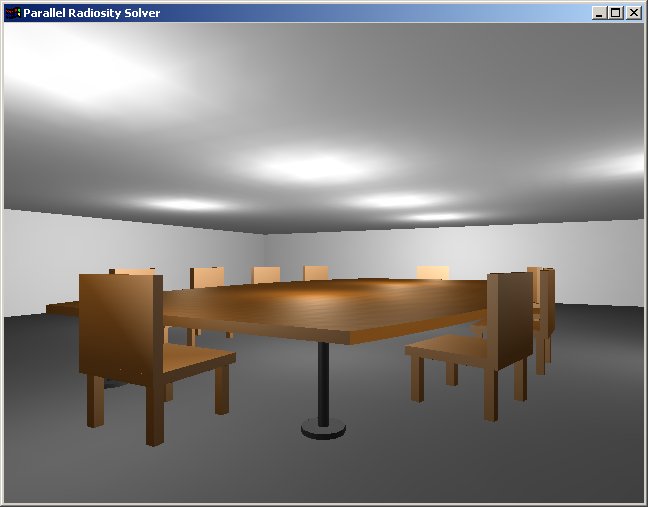
Here is the scene I originally built, which did undergo some modifications later:
Source Code
The following source code is in the public domain. Do whatever you want with it. I guarantee nothing about its correctness, readability, usefulness, or propensity to cause your computer to explode.
prad.cpp (frontend/client, runs on Windows)
rad-solver.cpp (server, runs on MPI)
rad-kernel.c (radiosity kernel for server, requires Intel
C compiler)
vector.h (used by both client and server)
Activities Not Yet Finished
Although the project due date is May 6 (extended now to May 8), I plan to do some additional work before the presentations (May 13/15) and the AUP due date (May 24). The AUP has a 10-page report required. Here are the remaining milestones I have set:
Copyright © 2002 by Matt Craighead