| Amay Champaneria | amayc@mit.edu |
Tracking objects is a hard problem in computer vision. Methods such as Kalman filtering have been used for tracking, but such methods can only model unimodal probability distributions and thus cannot form alternative hypotheses about the location of the object being tracked. To address this weakness, Isard and Blake (IJCV 1998) developed an algorithm called condensation. Condensation uses "factored sampling", in which a distribution of possible locations is represented by a randomly generated set. Because it uses a Monte-Carlo-like sampling method, this algorithm is well suited for parallel processing. I propose to implement condensation to take advantage of parallel architectures, which will allow faster processing of video sequences.
The input to my software is a video sequence and a model describing the object to track. The output is a sequence of locations, each corresponding to where the algorithm found the object in the frame. As a test and proof-of-concept, my system tracks a pen as it is being used to write. This is a good test case because it emphasizes the importance of alternative hypotheses: the writer's hand may block part of the pen, which would trip up traditional tracking algorithms such as Kalman filtering. Since condensation maintains multiple hypotheses, it should be robust against partial occlusions or momentary disappearances of the pen. This is also a good test case for me because it ties into my thesis work on handwriting recognition.
So far we have been getting up to speed by reading papers about the condensation algorithm and its applications. We have obtained some code for a simple application of condensation (tracking the motion of a scalar), and we are using this both to understand the algorithm and to serve as a model for our own implementation. We have set up a CVS source tree and are now writing a single-processor tracker in C. In parallel to our coding, we are also actively discussing how to parallelize the algorithm efficiently. So far, we have decided that the factored sampling step of the algorithm (the Monte Carlo part) will definitely be spread across all nodes, but we have yet to determine the communication pattern and whether other steps will be done in parallel. The next move will be to use MPI to parallelize our code. Then we must test and benchmark the system and (if necessary) tweak the load-balancing to improve performance. Though we have a lot of work ahead of us, we feel that we are off to a good start.
The condensation algorithm provides predictions of future measurements based on the conditional probability densities of past measurements. In the context of our project, the measurements are coordinates where we can expect to find the pen tip in a given frame. Condensation can be summarized as follows:
|
Define xt to be the state of the object being modelled (and tracked) at time t From the "old" sample-set { st-1[n], wt-1[n], ct-1[n], n=1..N } at time-step t-1, Construct the nth of N new samples as follows:
xmean(t) = Sum(wt[n] * st[n] over n) |
Basically, the algorithm produces more accurate results for more samples (higher N), and since the samples are highly independent, I decided that they should be run in parallel. After each iteration, the results must be shared across all nodes, so I must design a communication pattern that accomplishes this data sharing in an efficient manner. The software is written in C using MPI for intended use on the class Beowulf cluster.
My code consists of three significant modules: the frontend, the tracker, and the condensation filter. Each of these modules is described in detail below.
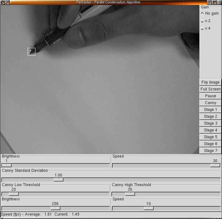
This module provides the user interface for the rest of the program. Both a GTK-based GUI and a command-line interface are provided. The GUI allows the user to record and view sequences of video frames and to see the results of the tracking. A screenshot of the GUI is displayed below. The command-line interface allows the user to perform the tracking on video sequences without the computational costs of a GUI display. Thus, the development cycle was basically to write and tweak the tracker using the GUI (to ensure that the tracking is accurate), and then to test the performance using the command-line interface.
The frontend code is organized as follows:
|
I obtained code for a pen-tracking system from Mario Munich and Pietro Perona of Caltech. Basically, I hacked this code to work with my video sequences.
The tracker code is organized as follows:
As described above, Munich's tracker was based on a Kalman filter. I replaced this with my own parallel version of Isard and Blake's Condensation filter. Though the general algorithm is explained above, I describe my parallel implementation in this section.
To facilitate understanding of my implementation, the following figure compares the original serial and my parallel version of the steady-state (after initialization) loop of the Condensation algorithm in the context of pen-tracking (pseudocode):| Serial Implementation | My Parallel Implementation |
condensation_filter()
{
  obtain_observations()
  predict_new_bases()
  calculate_base_weights()
  update_after_iterating()
}


predict_new_bases()
{
  for i = 0 to N
  {
    base = pick_base_sample()
    predict_sample_position(i, base)
  }
}


calculate_base_weights()
{
  cumulative_total = 0

  for i = 0 to N
  {
    sample_weights[i] = evaluate_observation_density(i)
    cumulative_probabilities[i] = cumulative_total
    cumulative_total += sample_weights[i]
  }
}
|
condensation_filter()
{
  obtain_observations()
predict_new_bases_and_observe() calculate_cumulative() update_after_iterating() }
// PARALLEL
predict_new_bases_and_observe()
{
  // split the N samples into num_nodes blocks
  nstart = N * rank/num_nodes
  nstop =  N * (rank+1)/num_nodes

  for i = nstart to nstop
  {
    base = pick_base_sample()
    predict_sample_position(i, base)
    sample_weights[i] = evaluate_observation_density(i);
  }
}
calculate_cumulative()
{
  cumulative_total = 0.0;

  for i = 0 to N
  {
    cumulative_probabilities[i] = cumulative_total;
    cumulative_total += sample_weights[i];
  }
}
|
| Red indicates steps done in parallel | |
Originally, I had planned on parallelizing only the factored sampling step of the algorithm (predict_new_bases from above), since it basically consists of obtaining N independent random samples. After implementing this, I found that the performance decreased as the number of nodes increased. Realizing that this result meant that predict_new_bases was too simple (thus I was spending a lot of communication to achieve very little computation), I decided to parallelize the observation step as well. The result was the new predict_new_bases_and_observe routine. Obtaining observations involves significantly more computation than predict_new_bases, and it can be done independently of other samples, which makes it a good candidate for parallel computation.
I experimented with a few different communication patterns and eventually settled upon having all nodes decompress the video frames on their own and having a "smart" root node in charge of dispatching computation to other nodes. Though decompressing each frame on each node leads to redundant computation, the alternatives seemed unattractive:
The decision to put the root node in charge of dispatching computation and gathering results from the other nodes was driven by the condensation algorithm itself. As discussed above, the original goal was to parallelize the factored sampling step, then gather the results back and determine a new prediction. Certain steps, such as calculate_cumulative, require serial processing so it makes sense to do this on the root node.
Though having a smart root node meant I could avoid costly all-to-all communication, it created a potential bottleneck at the root. Fortunately, I parallelized the right steps in the algorithm, so after receiving the results of the parallel computation, the root node has very simple tasks to do before the next iteration.
To summarize the messages passed in my parallel implementation, I'll step through the algorithm and outline the communication. At initialization, the root node acquires a model of the pen tip and broadcasts it along with other necessary data to the other nodes (all using MPI_Bcast). Upon receiving these data, the other nodes are ready to begin computation. In the steady-state loop of the algorithm, the root node obtains measurements of where the pen is in the current frame and broadcasts these to the other nodes (again using MPI_Bcast). With these measurements, all nodes sample independently and weight their new samples according to their likelihoods, and the resulting samples and weights are sent back to the root (MPI_Gather). Finally, the root node performs the serial steps of the algorithm and updates the other nodes via MPI_Bcast and the next iteration starts. Though this may seem like a lot of communication per iteration, it ends up speeding up the overall computation, as we'll see in the results section.
The parallel condensation filter is implemented in condensation.c.
My source code is available here: partrackersrc.tgz. You will probably find the tarball of my CVS tree, which includes this document, the Makefiles for each version of the tracker, and a sample video sequence, more useful: partrackercvs.tgz
To test the performance of my parallel tracker, I recorded a 513-frame video sequence of myself writing with a pen. I held the pen steady for the first 150 frames to allow the system to acquire a model of the pen tip. After the tip-acquisition period, I scribbled for about 350 frames, and then in the final frames I removed the pen from the scene to stop tracking. It's important to note that during the scribbling I deliberately wrote over previous pen strokes to test how robust the tracker is against cluttered backgrounds. As mentioned above, one of condensation's strengths is that it maintains tracking even in cluttered backgrounds, so I thought I would test that claim.
I evaluated the performance of my system in two aspects: speed and accuracy. To measure speed, I added profiling code to record the total time spent in the tracking stage for all frames tracked. Dividing the resulting figure by the number of frames tracked gave me the overall framerate of the tracker. I measured the framerate of the baseline Kalman tracker and my parallel Condensation tracker (partracker) under varied parameters. In testing the partracker, I varied the number of samples (N) from 100 to 100000--we would expect accuracy to increase and framerates to decrease as we increase N. I tested at the usual number of nodes: 1, 2, 4, 8, and 16. The results are shown in Figure 3.
 |
As you can see, the Kalman tracker is pretty fast already, at 73.6 frames per second (fps). At N=100, the partracker blazes through the frames at 100 fps on one node, but the performance drops as nodes are added. This makes some sense because we are only taking 100 samples, so splitting them to multiple nodes achieves very little computation at the expense of a lot of communication. At N=1000, partracker's performance peaks around 4 and 8, beating the Kalman tracker. As nodes increase past 4, we expect to see such a decrease in performance, as a broadcast now costs much more than before. The pattern follows for N=10000, for which the partracker peaks at 8 nodes. And at N=100000, it seems as though performance is slowly increasing as nodes are added. It would be interesting to see if this trend would continue if we tried it on more than 16 nodes.
Now we turn to accuracy. To generate the reference coordinates (ground truth), I modified the tracker to take the maximum correlation between the pen tip and the image at each point. Though this reference tracker was incredibly slow (less than 1 fps), it yielded accurate results which I then used to benchmark the other trackers. My measure for inverse accuracy (error) is the square root of the average squared difference between the experimental coordinates and the reference coordinates:
E = sqrt( Sum((xi - xrefi)2 over F)/F ) + sqrt( Sum((yi - yrefi)2 over F)/F ), where F = number of frames
I used this measure to approximate the average number of pixels that each tracker prediction was off from the reference position. In terms of accuracy, our results are encouraging. All runs of the partracker generated an error of 5.86, while the Kalman tracker generated an error of 8.67. So on average, the partracker was more accurate than the Kalman tracker. One mystery about these results is that the partracker's accuracy did not improve as N increased. We would have expected that more samples mean a higher resolution picture of the actual probability density of the tracked position and thus, a more accurate prediction. I speculate that the video sequence I used was too clear and easy-to-track for us to really see the robustness of the Condensation algorithm. I would have liked to try the partracker on a video sequence with more rapid movement and a more cluttered background, to test my speculation.
Videos of the tracking results are available below. Also, the perl script I wrote to evaluate the error for each run is available here: diffcoords.pl.
Clearly, we've seen that the parallel Condensation tracker not only works, but is more accurate than the baseline Kalman tracker and in certain conditions, is faster. From here, there are many other possibilities that I would suggest to explore: I would encourage anyone with an interest and some extra time to check out the source code and attempt one of these suggestions.
Last updated May 8, 2002 by amayc@mit.edu.6. Future Work
7. Downloads