To print these notes, use the PDF version.

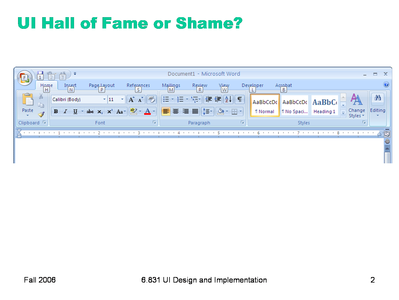
Our Hall of Fame or Shame candidate for today is the command ribbon, which was introduced in Microsoft Office 2007.  The ribbon is a radically different user interface for Office, merging the menubar and toolbars together into a single common widget.  Clicking on one of the tabs (“Write”, “Insert”, “Page Layout”, etc) switches to a different ribbon of widgets underneath.  The metaphor is a mix of menubar, toolbar, and tabbed pane.  (Notice how UIs have evolved to the point where new metaphorical designs are riffing on existing GUI objects, rather than physical objects.  Expect to see more of that in the future.)

Needless to say, slavish external consistency has been thrown out the window — Office no longer has a menubar or toolbar.  But if we were slavishly consistent, we’d never make any progress in user interface design.  Despite the radical change, the ribbon is still externally consistent in some interesting ways, with other Windows programs and with previous versions of Office.  Can you find some of those ways?

The ribbon is also notable for being designed from careful task analysis.  How can you tell?

Today’s lecture continues our look into the mechanics of implementing user interfaces, by considering output in more detail.

One goal for these implementation lectures is not to teach any one particular GUI system or toolkit, but to give a survey of the issues involved in GUI programming and the range of solutions adopted by various systems.  Presumably you’ve already encountered at least one GUI toolkit, probably Java Swing.  These lectures should give you a sense for what’s common and what’s unusual in the toolkit you already know, and what you might expect to find when you pick up another GUI toolkit.

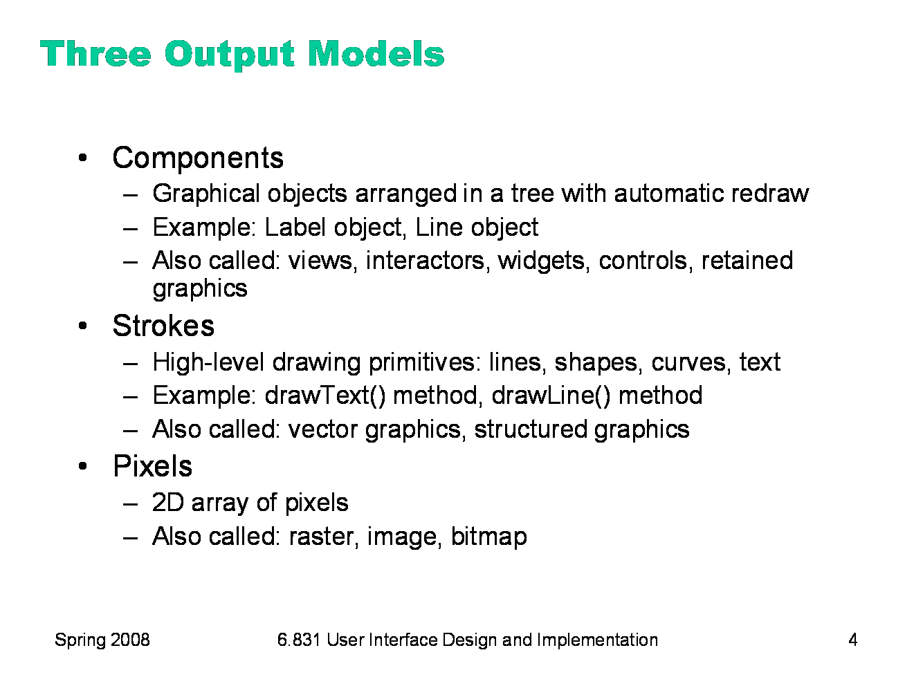
There are basically three ways to represent the output of a graphical user interface.

Components is the same as the view hierarchy we discussed last week.  Parts of the display are represented by view objects arranged in a spatial hierarchy, with automatic redraw propagating down the hierarchy.  There have been many names for this idea over the years; the GUI community hasn’t managed to settle on a single preferred term.

Strokes draws output by making calls to high-level drawing primitives, like drawLine, drawRectangle, drawArc, and drawText.

Pixels regards the screen as an array of pixels and deals with the pixels directly.

All three output models appear in virtually every modern GUI application.  The component model always appears at the very top level, for windows, and often for components within the windows as well.  At some point, we reach the leaves of the view hierarchy, and the leaf views draw themselves with stroke calls.  A graphics package then converts those strokes into pixels displayed on the screen. For performance reasons, a component may short-circuit the stroke package and draw pixels on the screen directly. On Windows, for example, video players do this using the DirectX interface to have direct control over a particular screen rectangle.

What model do each of the following representations use?  HTML (component); Postscript laser printer (stroke input, pixel output); plotter (stroke input and output); PDF (stroke); LCD panel (pixel).

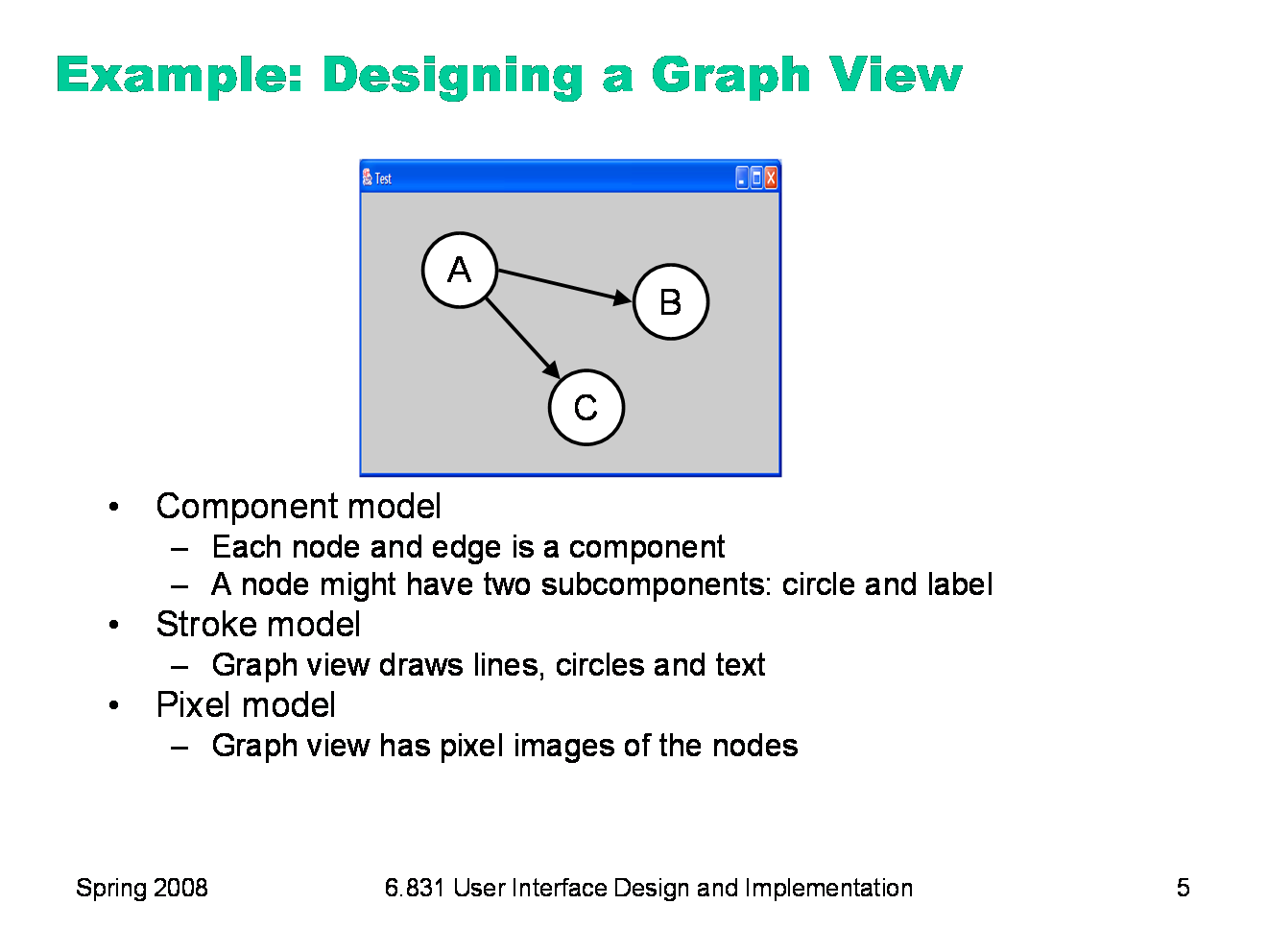
Since every application uses all three models, the design question becomes: at which points in your application do you want to step down into a lower-level output model?  Here’s an example.  Suppose you want to build a view that displays a graph of nodes and edges.

One approach would represent each node and each edge in the graph by a component. Each node in turn might have two components, a circle and a text label.  Eventually, you’ll get down to the primitive components available in your GUI toolkit.  Most GUI toolkits provide a text label component; most don’t provide a primitive circle component.  One notable exception is Amulet, which has component equivalents for all the common drawing primitives.  This would be a pure component model, at least from your application’s point of view — stroke output and pixel output would still happen, but inside primitive components that you took from the library.

Alternatively, the top-level window might have no subcomponents.  Instead, it would draw the entire graph by a sequence of stroke calls: drawCircle for the node outlines, drawText for the labels, drawLine for the edges.  This would be a pure stroke model.

Finally, your graph view might bypass stroke drawing and set pixels in the window directly.  The text labels might be assembled by copying character images to the screen.  This pure pixel model is rarely used nowadays, because it’s the most work for the programmer, but it used to be the only way to program graphics.

Hybrid models for the graph view are certainly possible, in which some parts of the output use one model, and others use another model.  The graph view might use components for nodes, but draw the edges itself as strokes.  It might draw all the lines itself, but use label components for the text.

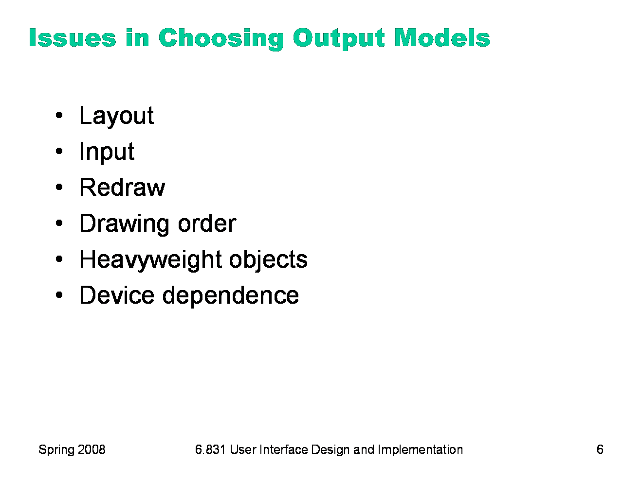
Layout: Components remember where they were put, and draw themselves there.  They also support automatic layout.  With stroke or pixel models, you have to figure out (at drawing time) where each piece goes, and put it there.

Input: Components participate in event dispatch and propagation, and the system automatically does hit-testing (determining whether the mouse is over the component when an event occurs) for components, but not for strokes.  If a graph node is a component, then it can receive its own click and drag events.  If you stroked the node instead, then you have to write code to determine which node was clicked or dragged.

Redraw: An automatic redraw algorithm means that components redraw themselves automatically when they have to.  Furthermore, the redraw algorithm is efficient: it only redraws components whose extents intersect the damaged region.  The stroke or pixel model would have to do this test by hand.  In practice, most stroked components don’t bother, simply redrawing everything whenever some part of the view needs to be redrawn.

Drawing order: It’s easy for a parent to draw before (underneath) or after (on top of) all of its children.  But it’s not easy to interleave parent drawing with child drawing.  So if you’re using a hybrid model, with some parts of your view represented as components and others as strokes, then the components and strokes generally fall in two separate layers, and you can’t have any complicated z-ordering relationships between strokes and components.

Heavyweight objects: Every component must be an object (and even an object with no fields costs about 20 bytes in Java). As we’ve seen, the view hierarchy is overloaded not just with drawing functions but also with event dispatch, automatic redraw, and automatic layout, so that further bulks up the class.  The flyweight pattern used by InterView’s Glyphs can reduce this cost somewhat.  But views derived from large amounts of data — say, a 100,000-node graph — generally can’t use a component model.

Device dependence: The stroke model is largely device independent.  In fact, it’s useful not just for displaying to screens, but also to printers, which have dramatically different resolution.  The pixel model, on the other hand, is extremely device dependent.  A directly-mapped pixel image won’t look the same on a screen with a different resolution.

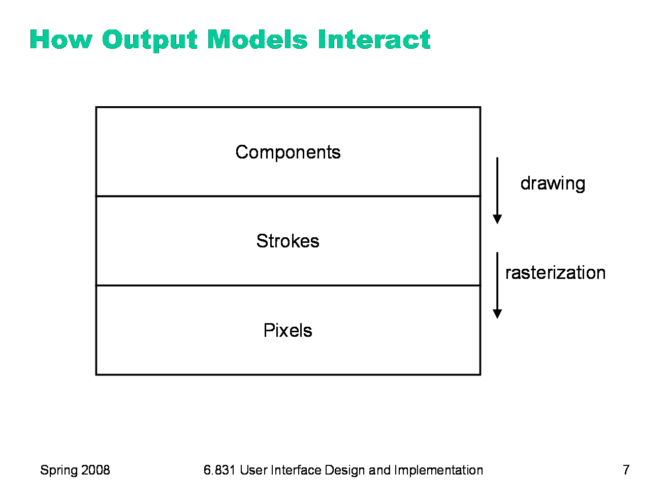
As we said earlier, almost every GUI program uses all three models.  At the highest level, a typical program presents itself in a window, which is a component.  At the lowest level, the window appears on the screen as a rectangle of pixels.  So a series of steps has to occur that translates that window component (and all the components it contains) into pixels.

The step from the component model down to the stroke model is usually called drawing.  We’ll look at that first.

The step from strokes down to pixels is called rasterization (or scan conversion). The specific algorithms that rasterize various shapes are beyond the scope of this course (see 6.837 Computer Graphics instead).  But we’ll talk about some of the effects of rasterization, and what you need to know as a UI programmer to control those effects.

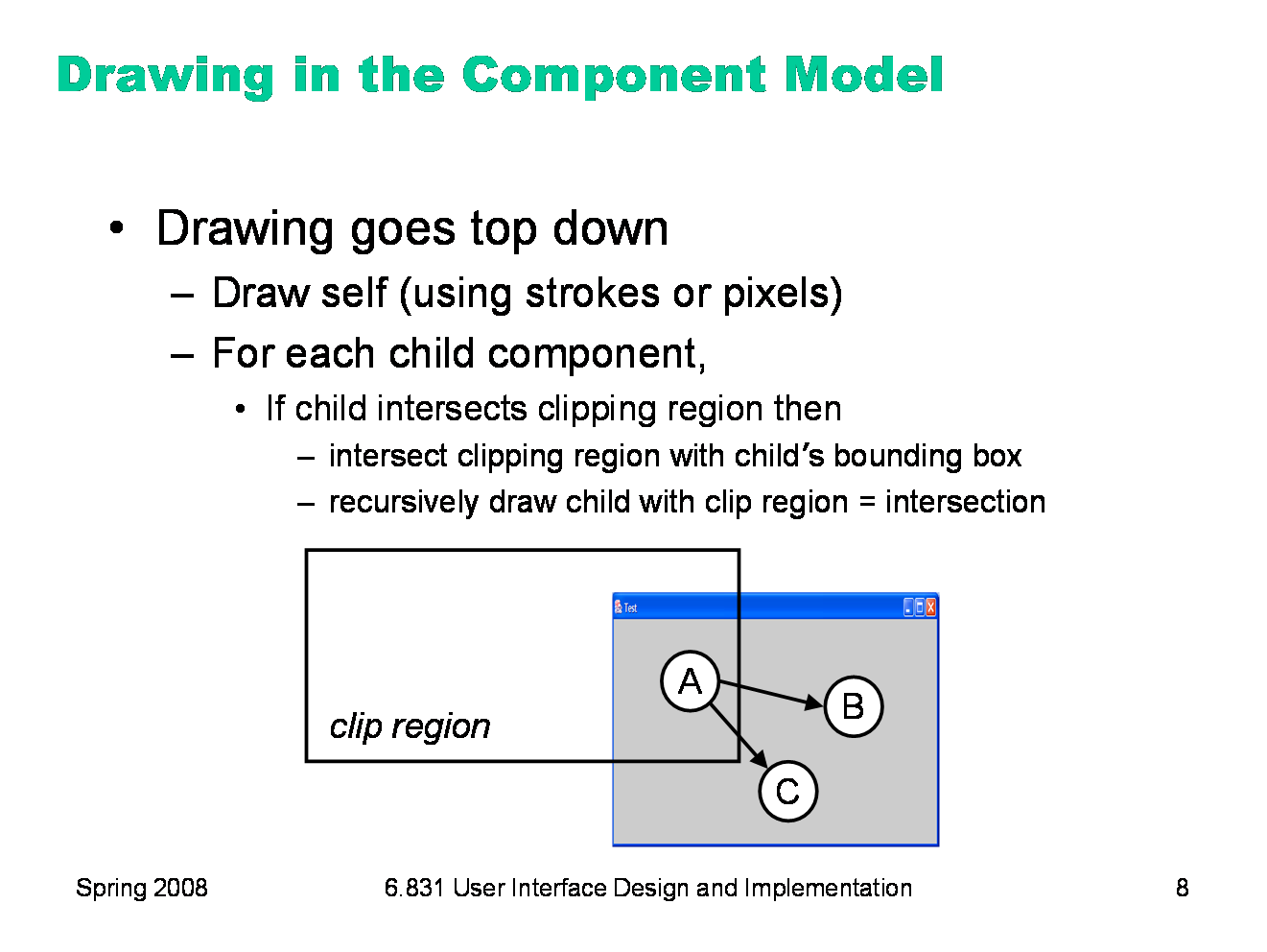
Here’s how drawing works in the component model.  Drawing is a top-down process: starting from the root of the component tree, each component draws itself, then draws each of its children recursively.  The process is optimized by passing a clipping region to each component, indicating the area of the screen that needs to be drawn.  Child components that do not intersect the clipping region are simply skipped, not drawn. In the example above, nodes B and C would not need to be drawn.  When a component partially intersects the clipping region, it must be drawn — but any strokes or pixels it draws when the clipping region is in effect will be masked against the clip region, so that only pixels falling inside the region actually make it onto the screen.

For the root component, the clipping region might be the entire screen.  As drawing descends the component tree, however, the clipping region is intersected with each component’s bounding box.  So the clipping region for a component deep in the tree is the intersection of the bounding boxes of its ancestors.

For high performance, the clipping region is normally rectangular, using component bounding boxes rather than the components’ actual shape.  But it doesn’t have to be that way.  A clipping region can be an arbitrary shape on the screen.  This can be very useful for visual effects: e.g., setting a string of text as your clipping region, and then painting an image through it like a stencil.  Postscript was the first stroke model to allow this kind of nonrectangular clip region. Now many graphics toolkits support nonrectangular clip regions. For example, on Microsoft Windows and X Windows, you can create nonrectangular windows, which clip their children into a nonrectangular region.

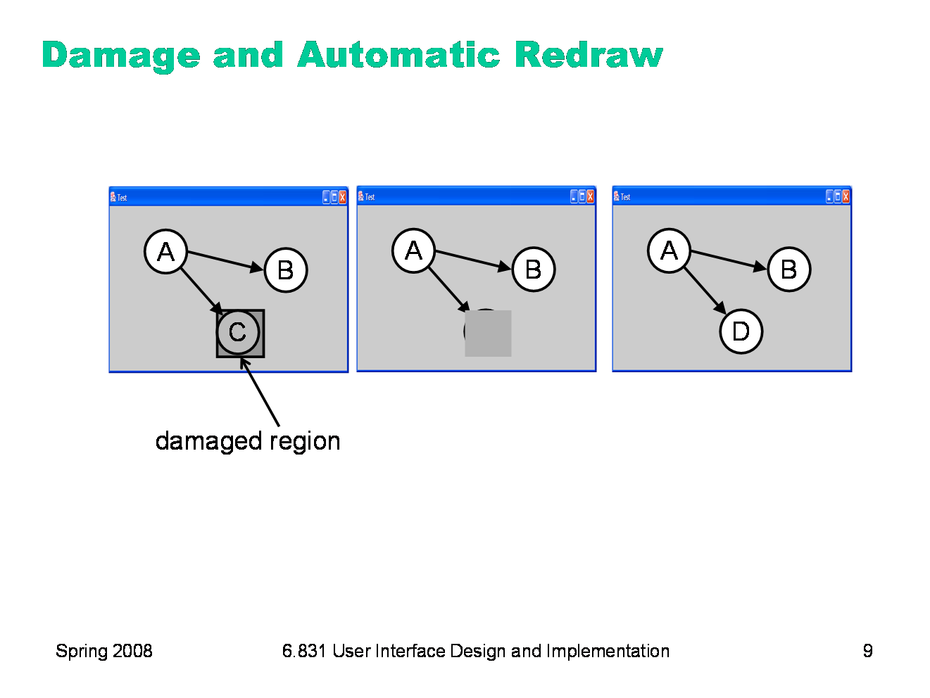
When a component needs to change its appearance, it doesn’t repaint itself directly.  It can’t, because the drawing process has to occur top-down through the component hierarchy: the component’s ancestors and older siblings need to have a chance to paint themselves underneath it.  (So, in Java, even though a component can call its own paint() method directly, you generally shouldn’t do it!)

Instead, the component asks the graphics system to repaint it at some time in the future.  This request includes a damaged region, which is the part of the screen that needs to be repainted.  Often, this is just the entire bounding box of the component; but complex components might figure out which part of the screen corresponds to the part of the model that changed, so that only that part is damaged.

The repaint request is then queued for later.  Multiple pending repaint requests from different components are consolidated into a single damaged region, which is often represented just as a rectangle — the bounding box of all the damaged regions requested by individual components.  That means that undamaged screen area is being considered damaged, but there’s a tradeoff between the complexity of the damaged region representation and the cost of repainting.

Eventually — usually after the system has handled all the input events (mouse and keyboard) waiting on the queue -- the repaint request is finally satisfied, by setting the clipping region to the damaged region and redrawing the component tree from the root.

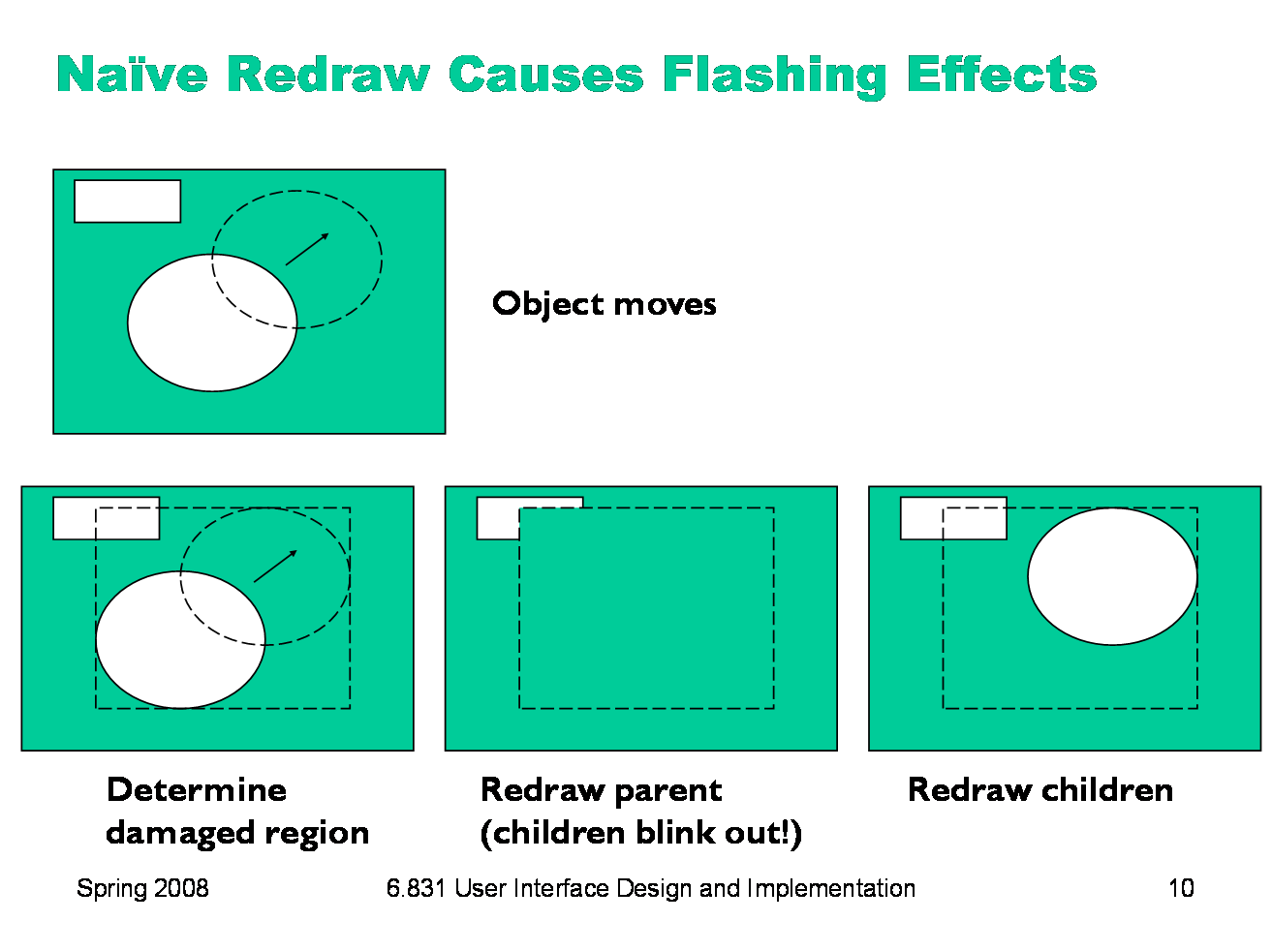
There’s an unfortunate side-effect of the automatic damage/redraw algorithm. If we draw a component tree directly to the screen, then moving a component can make the screen appear to flash — objects flickering while they move, and nearby objects flickering as well.

When an object moves, it needs to be erased from its original position and drawn in its new position.  The erasure is done by redrawing all the objects in the view hierarchy that intersect this damaged region. If the drawing is done directly on the screen, this means that all the objects in the damaged region temporarily disappear, before being redrawn.  Depending on how screen refreshes are timed with respect to the drawing, and how long it takes to draw a complicated object or multiple layers of the hierarchy, these partial redraws may be briefly visible on the monitor, causing a perceptible flicker.

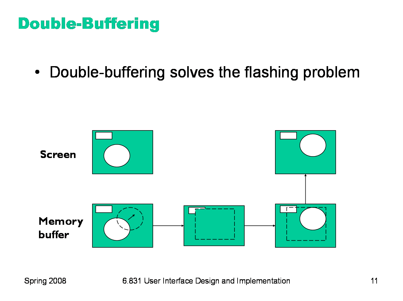
Double-buffering solves this flickering problem.  An identical copy of the screen contents is kept in a memory buffer.  (In practice, this may be only the part of the screen belonging to some subtree of the view hierarchy that cares about double-buffering.)  This memory buffer is used as the drawing surface for the automatic damage/redraw algorithm. After drawing is complete, the damaged region is just copied to screen as a block of pixels.  Double-buffering reduces flickering for two reasons: first, because the pixel copy is generally faster than redrawing the view hierarchy, so there’s less chance that a screen refresh will catch it half-done; and second, because unmoving objects that happen to be caught, as innocent victims, in the damaged region are never erased from the screen, only from the memory buffer.

It’s a waste for every individual view to double-buffer itself.  If any of your ancestors is double-buffered, then you’ll derive the benefit of it. So double-buffering is usually applied to top-level windows.

Why is it called double-buffering?  Because it used to be implemented by two interchangeable buffers in video memory.  While one buffer was showing, you’d draw the next frame of animation into the other buffer.  Then you’d just tell the video hardware to switch which buffer it was showing, a very fast operation that required no copying and was done during the CRT’s vertical refresh interval so it produced no flicker at all. 

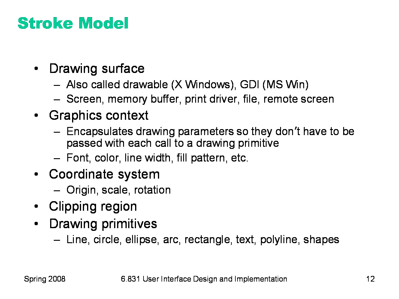
We’ve already considered the component model in some detail.  So now, let’s look at the stroke model.

Every stroke model has some notion of a drawing surface. The screen is only one possible place where drawing might go. Another common drawing surface is a memory buffer, which is an array of pixels just like the screen.  Unlike the screen, however, a memory buffer can have arbitrary dimensions.  The ability to draw to a memory buffer is essential for double-buffering.  Another target is a printer driver, which forwards the drawing instructions on to a printer.  Although most printers have a pixel model internally (when the ink actually hits the paper), the driver often uses a stroke model to communicate with the printer, for compact transmission.  Postscript, for example, is a stroke model.

Most stroke models also include some kind of a graphics context, an object that bundles up drawing parameters like color, line properties (width, end cap, join style), fill properties (pattern), and font.

The stroke model may also provide a current coordinate system, which can be translated, scaled, and rotated around the drawing surface.  We’ve already discussed the clipping region, which acts like a stencil for the drawing.  Finally, a stroke model must provide a set of drawing primitives, function calls that actually produce graphical output.

Many systems combine all these responsibilities into a single object.  Java’s Graphics object is a good example of this approach.  In other toolkits, the drawing surface and graphics context are independent objects that are passed along with drawing calls.

When state like graphics context, coordinate system, and clipping region are embedded in the drawing surface, the surface must provide some way to save and restore the context.  A key reason for this is so that parent views can pass the drawing surface down to a child’s draw method without fear that the child will change the graphics context.  In Java, for example, the context can be saved by Graphics.create(), which makes a copy of the Graphics object.  Notice that this only duplicates the graphics context; it doesn’t duplicate the drawing surface, which is still the same.

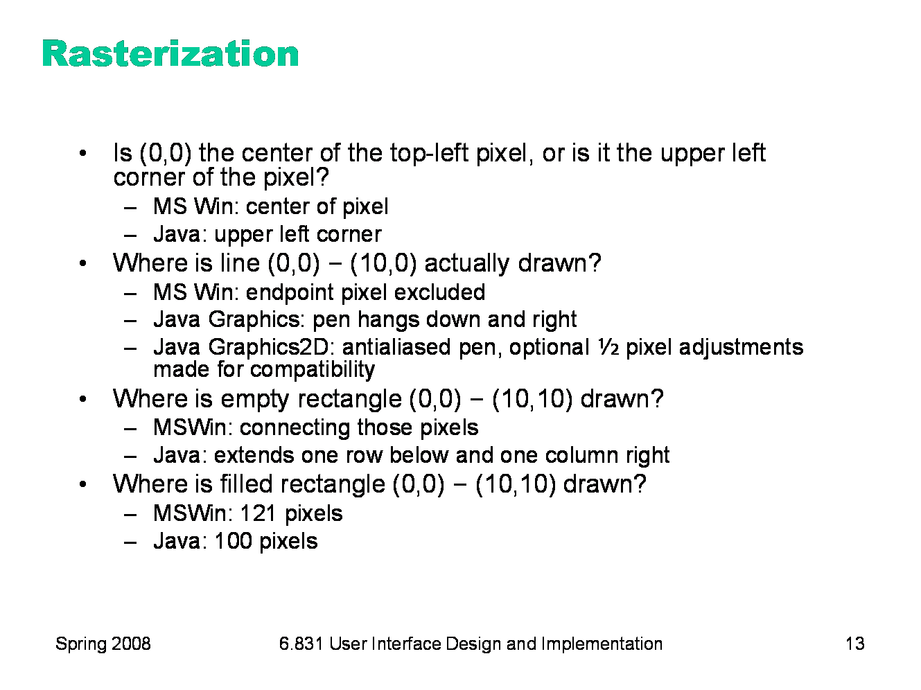
When you’re using a stroke model, it’s important to understand how the strokes are actually converted into pixels.  Different platforms make different choices.

One question concerns how stroke coordinates, which represent zero-dimensional points, are translated into pixel coordinates, which are 2-dimensional squares.  Microsoft Windows places the stroke coordinate at the center of the corresponding pixel; Java’s stroke model places the stroke coordinates between pixels.

The other questions concern which pixels are actually drawn when you request a line or a rectangle.

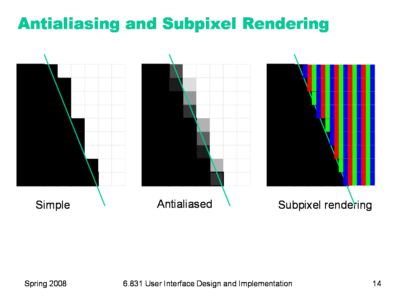
It’s beyond the scope of this lecture to talk about algorithms for converting a stroke into pixels.  But you should be aware of some important techniques for making strokes look good.

One of these techniques is antialiasing, which is a way to make an edge look smoother.  Instead of making a binary decision between whether to color a pixel black or white, antialiasing uses a shade of gray whose value varies depending on how much of the pixel is covered by the edge.  In practice, the edge is between two arbitrary colors, not just black and white, so antialiasing chooses a point on the gradient between those two colors.  The overall effect is a fuzzier but smoother edge.

Subpixel rendering takes this a step further.  Every pixel on an LCD screen consists of three discrete pixels side-by-side: red, green, and blue.  So we can get a horizontal resolution which is three times the nominal pixel resolution of the screen, simply by choosing the colors of the pixels along the edge so that the appropriate subpixels are light or dark.  It only works on LCD screens, not CRTs, because CRT pixels are often arranged in triangles, and because CRTs are analog, so the blue in a single “pixel” usually consists of a bunch of blue phosphor dots interspersed with green and red phosphor dots.  You also have to be careful to smooth out the edge to avoid color fringing effects on perfectly vertical edges.  And it works best for high-contrast edges, like this edge between black and white.  Subpixel rendering is ideal for text rendering, since text is usually small, high-contrast, and benefits the most from a boost in horizontal resolution.  Windows XP includes ClearType, an implementation of subpixel rendering for Windows fonts.  (For more about subpixel rendering, see Steve Gibson, “Sub-Pixel Font Rendering Technology”, http://grc.com/cleartype.htm)

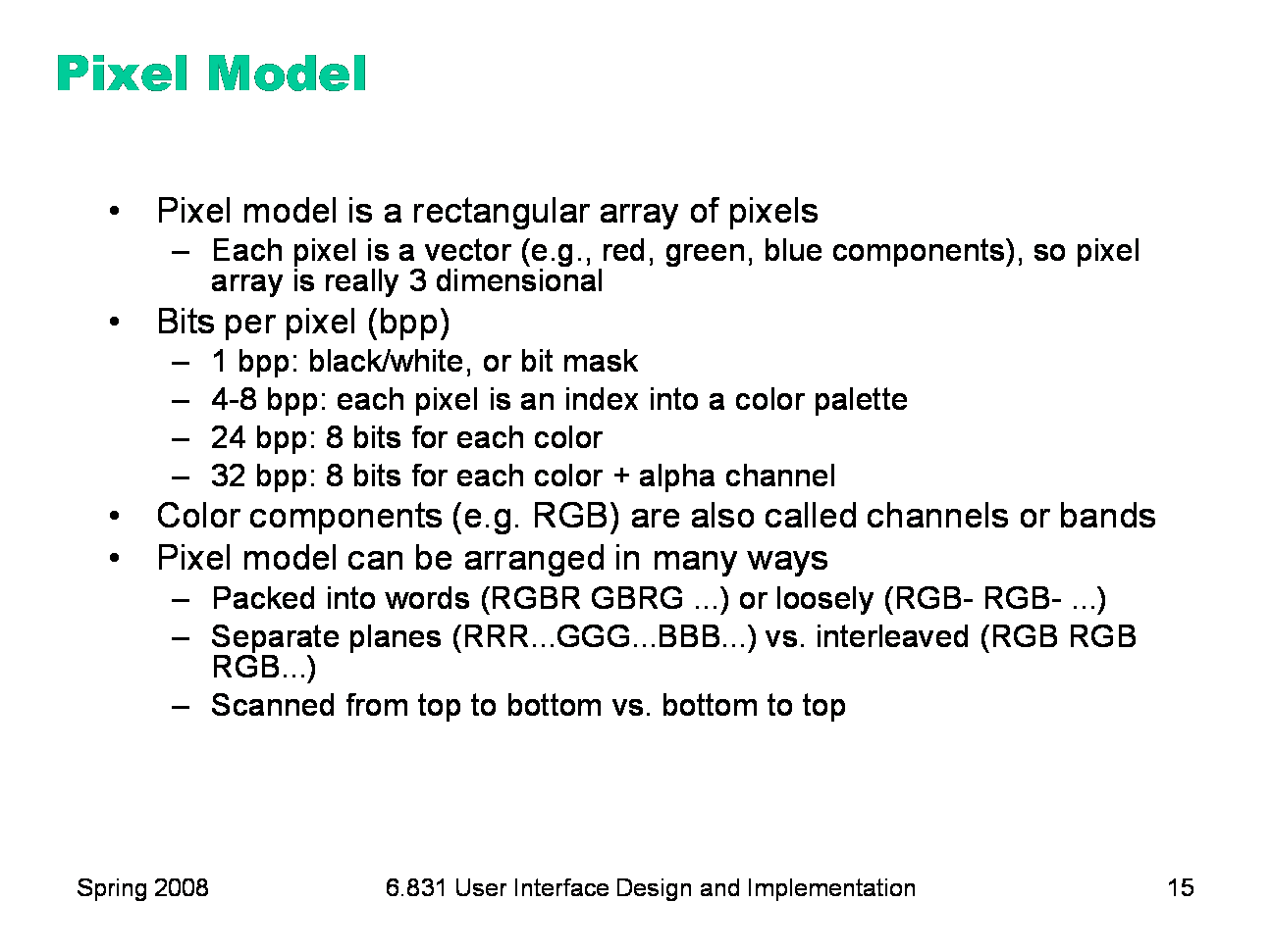
Finally, let’s talk in more detail about what the pixel model looks like.

Put simply, it’s a rectangular array of pixels — but pixels themselves are not always so simple.  A pixel itself has a depth, so this model is really three dimensional. Depth is often expressed in bits per pixel (bpp).  The simplest kind of pixel model has 1 bit per pixel; this is suitable for representing black and white images.  It’s also used for bitmasks, where the single-bit pixels are interpreted as boolean values (pixel present or pixel missing).  Bitmasks are useful for clipping — you can think of a bitmask as a stencil.

Another kind of pixel representation uses each pixel value as an index into a palette, which is just a list of colors.  In the 4-bpp model, for example, each of the 16 possible pixel values represents a different color.  This kind of representation, often called Indexed Color, was useful when memory was scarce; you still see it in the GIF file format, but otherwise it isn’t used much today.

The most common pixel representation is often called “true color” or “direct color”; in this model, each pixel represents a color directly.  The color value is usually split up into multiple components: red, green, and blue.  (Color components are also called channels or bands; the red channel of an image, for example, is a rectangular array of the red values of its pixels.)

A pixel model can be arranged in memory (or a file) in various ways: packed tightly together to save memory, or spread out loosely for faster access; with color components interleaved or separated; and scanned from the top (so that the top-left pixel appears first) or the bottom (the bottom-left pixel appearing first).

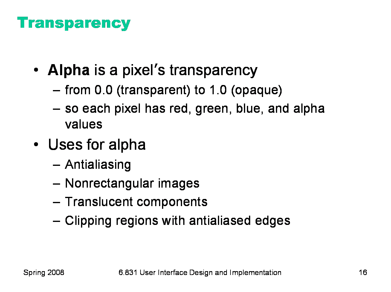
Many pixel models have a fourth channel in addition to red, green, and blue: the pixel’s alpha value, which represents its degree of transparency.  We’ll talk more about alpha in a future lecture.

The primary operation in the pixel model is copying a block of pixels from one place to another — often called bitblt (pronounced “bit blit”).  This is used for drawing pictures and icons on the screen, for example.  It’s also used for double-buffering — after the offscreen buffer is updated, its contents are transferred to the screen by a bitblt.

Bitblt is also used for screen-to-screen transfers.  To do fast scrolling, for example, you can bitblt the part of the window that doesn’t change upwards or downwards, to save the cost of redrawing it.  (For example, look at JViewport.BLIT_SCROLL_MODE.)

It’s also used for sophisticated drawing effects.  You can use bitblt to combine two images together, or to combine an image with a mask, in order to clip it or composite them together.

Bitblt isn’t always just a simple array copy operation that replaces destination pixels with source pixels.  There are various different rules for combining the destination pixels with the source pixels.  These rules are called compositing (alpha compositing, when the images have an alpha channel), and we’ll talk about them in a later lecture.

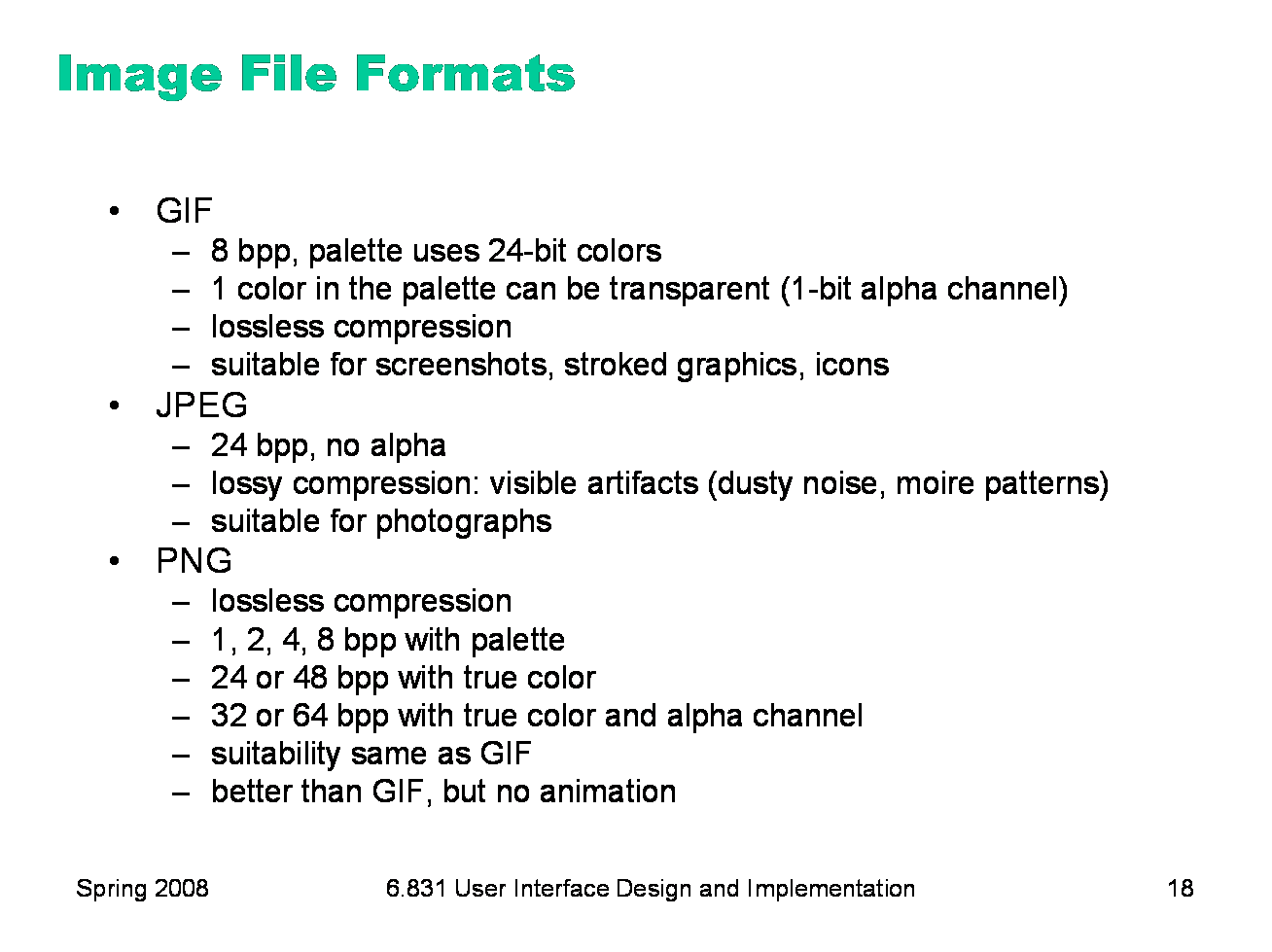
Here are a few common image file formats.  It’s important to understand when to use each format.  For user interface graphics, like icons, JPG generally should not be used, because it’s lossy compression — it doesn’t reproduce the original image exactly.  When every pixel matters, as it does in an icon, you don’t want lossy compression.  JPG also can’t represent transparent pixels, so a JPG image always appears rectangular in your interface.

For different reasons, GIF is increasingly unsuitable for interface graphics.  GIF isn’t lossy — you get the same image back from the GIF file that you put into it — but its color space is very limited.  GIF images use 8-bit color, which means that there can be at most 256 different colors in the image.  That’s fine for some low-color icons, but not for graphics with gradients or blurs.  GIF has limited support for transparency — pixels can either be opaque (alpha 1) or transparent (alpha 0), but not translucent (alpha between 0 and 1).  So you can’t have fuzzy edges in a GIF file, that blend smoothly into the background.  GIF files can also represent simple animations.

PNG is the best current format for interface graphics.  It supports a variety of color depths, and can have a full alpha channel for transparency and translucency.  (Unfortunately Internet Explorer 6 doesn’t correctly display transparent PNG images, so GIF still rules web graphics.) 

If you want to take a screenshot, PNG is the best format to store it.

Debugging output can sometimes be tricky.  A common problem is that you try to draw something, but it never appears on the screen.  Here are some possible reasons why.

Wrong place: what’s the origin of the coordinate system? What’s the scale?  Where is the component located in its parent?

Wrong size: if a component has zero width and zero height, it will be completely invisible no matter what it tries to draw— everything will be clipped.  Zero width and zero height are the defaults for all components in Swing — you have to use automatic layout or manual setting to make it a more reasonable size.  Check whether the component (and its ancestors) have nonzero sizes.

Wrong color: is the drawing using the same color as the background?  Is it using 100% alpha?

Wrong z-order: is something else drawing on top?